2 Software installation and first steps
Edited by: T. Hengl
This section contains instructions on how to install and use software to run predictive soil mapping and export results to GIS or web applications. It has been written (as has most of the book) for Linux users, but should not be too much of a problem to adapt to Microsoft Windows OS and/or Mac OS.
2.1 List of software in use
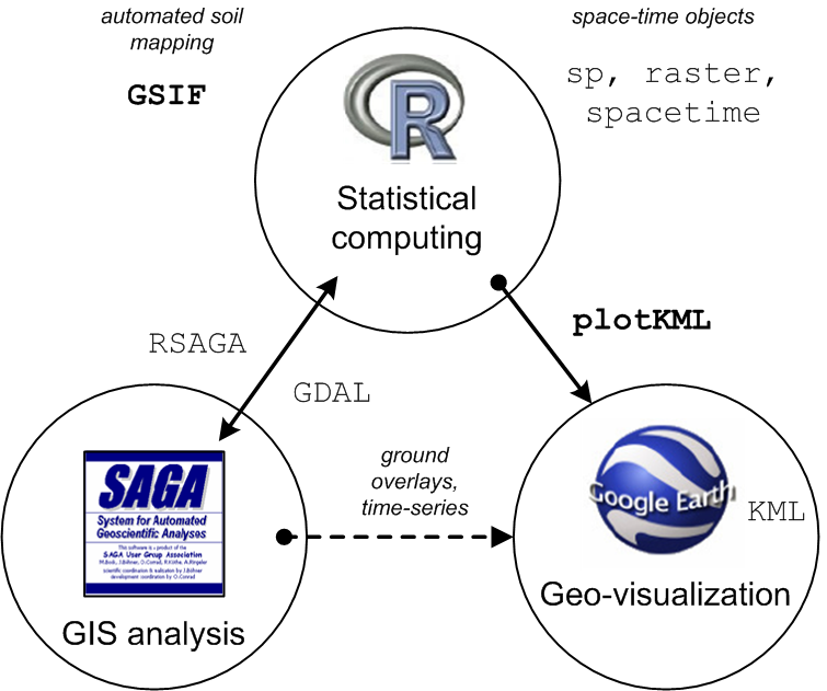
Figure 2.1: Software combination used in this book.
For processing the covariates we used a combination of Open Source GIS software, primarily SAGA GIS (Conrad et al. 2015), packages raster (Hijmans and van Etten 2017), sp (Pebesma and Bivand 2005), and GDAL (Mitchell and GDAL Developers 2014) for reprojecting, mosaicking and merging tiles. GDAL and parallel packages in R are highly suitable for processing large volumes of data.
Software required to run all exercises in the book includes:
R packages: GSIF, plotKML, aqp, ranger, caret, xgboost, plyr, raster, gstat, randomForest, ggplot2, e1071 (see: how to install R package)
SAGA GIS (on Windows machines run windows installer);
Google Earth or Google Earth Pro;
QGIS;
GDAL v2.x for Windows machines use e.g. “gdal-*-1800-x64-core.msi“;
R script used in this tutorial can be downloaded from github. As a gentle introduction to the R programming language and to soil classes in R we recommend the section 3.7 on importing and using soil data. Some more examples of SAGA GIS + R usage can be found in the soil covariates chapter. To visualize spatial predictions in a web-browser or Google Earth you can try using plotKML package (Hengl, Roudier, et al. 2015). As a gentle introduction to the R programming language and spatial classes in R we recommend following the Geocomputation with R book. Obtaining the R reference card is also highly recommended.
2.2 Installing software on Ubuntu OS
On Ubuntu (often the preferred standard for the GIS community) the main required software can be installed within 10–20 minutes. We start with installing GDAL, proj4 and some packages that you might need later on:
sudo apt-get install libgdal-dev libproj-dev
sudo apt-get install gdal-bin python-gdal
Next, we install R and RStudio. For R studio you can use the CRAN distribution or the optimized distribution provided by the former REvolution company (now owned by Microsoft):
wget https://mran.blob.core.windows.net/install/mro/3.4.3/microsoft-r-open-3.4.3.tar.gz
tar -xf microsoft-r-open-3.4.3.tar.gz
cd microsoft-r-open/
sudo ./install.sh
Note that R versions are constantly being updated so you will need to replace the URL above based on the most current information provided on the home page (http://mran.microsoft.com). Once you run install.sh you will have to accept the license terms twice before the installation can be completed. If everything completes successfully, you can get the session info by typing:
sessionInfo()
#> R version 3.5.2 (2017-01-27)
#> Platform: x86_64-pc-linux-gnu (64-bit)
#> Running under: Ubuntu 14.04.5 LTS
#>
#> Matrix products: default
#> BLAS: /home/travis/R-bin/lib/R/lib/libRblas.so
#> LAPACK: /home/travis/R-bin/lib/R/lib/libRlapack.so
#>
#> locale:
#>  [1] LC_CTYPE=en_US.UTF-8       LC_NUMERIC=C
#>  [3] LC_TIME=en_US.UTF-8        LC_COLLATE=en_US.UTF-8
#>  [5] LC_MONETARY=en_US.UTF-8    LC_MESSAGES=en_US.UTF-8
#>  [7] LC_PAPER=en_US.UTF-8       LC_NAME=C
#>  [9] LC_ADDRESS=C               LC_TELEPHONE=C
#> [11] LC_MEASUREMENT=en_US.UTF-8 LC_IDENTIFICATION=C
#>
#> attached base packages:
#> [1] stats     graphics  grDevices utils     datasets  methods   base
#>
#> other attached packages:
#> [1] knitr_1.21           microbenchmark_1.4-6
#>
#> loaded via a namespace (and not attached):
#>  [1] compiler_3.5.2   magrittr_1.5     bookdown_0.9     tools_3.5.2
#>  [5] htmltools_0.3.6  yaml_2.2.0       Rcpp_1.0.0       codetools_0.2-15
#>  [9] stringi_1.2.4    rmarkdown_1.11   highr_0.7        stringr_1.3.1
#> [13] xfun_0.5 digest_0.6.18 evaluate_0.12system("gdalinfo --version")This shows, for example, that the this installation of R is based on the Ubuntu 16.* LTS operating system and the version of GDAL is up to date. Using an optimized distribution of R (read more about “The Benefits of Multithreaded Performance with Microsoft R Open”) is especially important if you plan to use R for production purposes i.e. to optimize computing and generation of soil maps for large numbers of pixels.
To install RStudio we can run:
sudo apt-get install gdebi-core
wget https://download1.rstudio.org/rstudio-1.1.447-amd64.deb
sudo gdebi rstudio-1.1.447-amd64.deb
sudo rm rstudio-1.1.447-amd64.deb
Again, RStudio is constantly updated so you might have to obtain the most recent RStudio version and distribution. To learn more about doing first steps in R and RStudio and to learn to improve your scripting skills more efficiently, consider studying the following tutorials:
Grolemund, G., (2014) Hands-On Programming with R. O’Reilly, 236 pages.
Gillespie, C., Lovelace, R., (2016) Efficient R programming. O’Reilly, 222 pages.
Wilke, C.O., (2019) Fundamentals of Data Visualization. O’Reilly, in press.
2.3 Installing GIS software
Predictive soil mapping is about making maps, and working with maps requires use of GIS software to open, view overlay and analyze the data spatially. GIS software recommended in this book for soil mapping consists of SAGA GIS, QGIS, GRASS GIS and Google Earth. QGIS comes with an extensive literature and can be used to publish maps and combine layers served by various organizations. SAGA GIS, being implemented in C++, is highly suited for running geoprocessing on large data sets. To install SAGA GIS on Ubuntu we can use:
sudo add-apt-repository ppa:ubuntugis/ubuntugis-unstable
sudo apt-get update
sudo apt-get install saga
If installation is successful, you should be able to access SAGA command line also from R by using:
system("saga_cmd --version")To install QGIS (https://download.qgis.org/) you might first have to add the location of the debian libraries:
sudo sh -c 'echo "deb http://qgis.org/debian xenial main" >> /etc/apt/sources.list'
sudo sh -c 'echo "deb-src http://qgis.org/debian xenial main " >> /etc/apt/sources.list'
sudo apt-get update
sudo apt-get install qgis python-qgis qgis-plugin-grass
Other utility software that you might need include htop program that allows you to track processing progress:
sudo apt-get install htop iotopand some additional libraries use devtools, geoR and similar, which can be installed via:
sudo apt-get install build-essential automake;
        libcurl4-openssl-dev pkg-config libxml2-dev;
        libfuse-dev mtools libpng-dev libudunits2-dev
You might also need the 7z software for easier compression and pigz for parallelized compression:
sudo apt-get install pigz zip unzip p7zip-full 2.4 WhiteboxTools
WhiteboxTools (http://www.uoguelph.ca/~hydrogeo/WhiteboxTools/), contributed by John Lindsay, is an extensive suite of functions and tools for DEM analysis which is especially useful for extending the hydrological and morphometric analysis tools available in SAGA GIS and GRASS GIS (Lindsay 2016). Probably the easiest way to use WhiteboxTools is to install a QGIS plugin (kindly maintained by Alexander Bruy: https://plugins.bruy.me/) and then learn and extend the WhiteboxTools scripting language by testing things out in QGIS (see below).
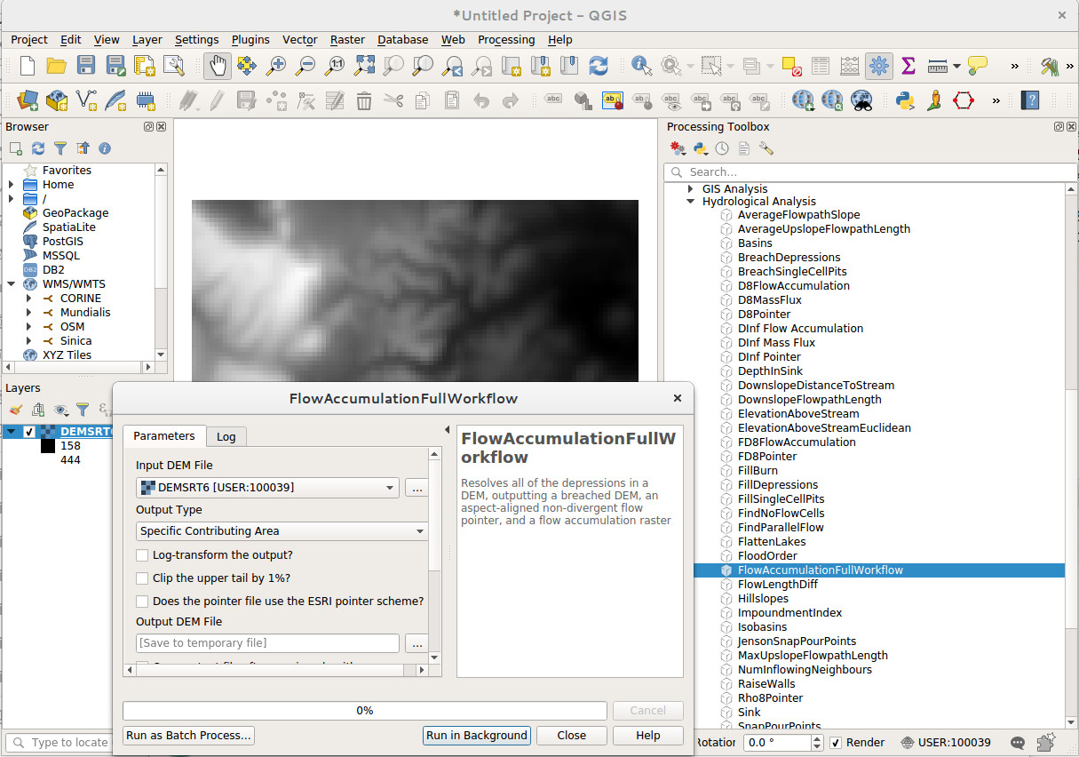
Figure 2.2: Calling WhiteboxTools from QGIS via the WhiteboxTools plugin.
The function FlowAccumulationFullWorkflow is, for example, a wrapper function to filter out all spurious sinks and to derive a hydrological flow accumulation map in one step. To run it from command line we can use:
system(paste0('"/home/tomislav/software/WBT/whitebox_tools" ',
  '--run=FlowAccumulationFullWorkflow --dem="./extdata/DEMTOPx.tif" ',
  '--out_type="Specific Contributing Area" --log="False" --clip="False" ',
  '--esri_pntr="False" ',
  '--out_dem="./extdata/DEMTOPx_out.tif" ',
  '--out_pntr="./extdata/DEMTOPx_pntr.tif" ',
  '--out_accum="./extdata/DEMTOPx_accum.tif" -v'))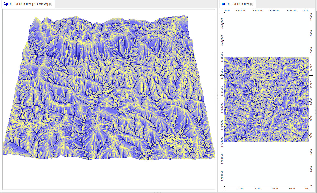
Figure 2.3: Hydrological flow accummulation map based on the Ebergotzen DEM derived using WhiteboxTools.
This produces a number of maps, from which the hydrological flow accumulation map is usually the most useful. It is highly recommended that, before running analysis on large DEM’s using WhiteboxTools and/or SAGA GIS, you test functionality using smaller data sets i.e. either a subset of the original data or using a DEM at very coarse resolution (so that width and height of a DEM are only few hundred pixels). Also note that WhiteboxTools do not presently work with GeoTIFs that use the COMPRESS=DEFLATE creation options.
2.5 RStudio
RStudio is, in principle, the main R scripting environment and can be used to control all other software used in this tutorial. A more detailed RStudio tutorial is available at: RStudio — Online Learning. Consider also following some spatial data tutorials e.g. by James Cheshire (http://spatial.ly/r/). Below is an example of an RStudio session with R editor on right and R console on left.
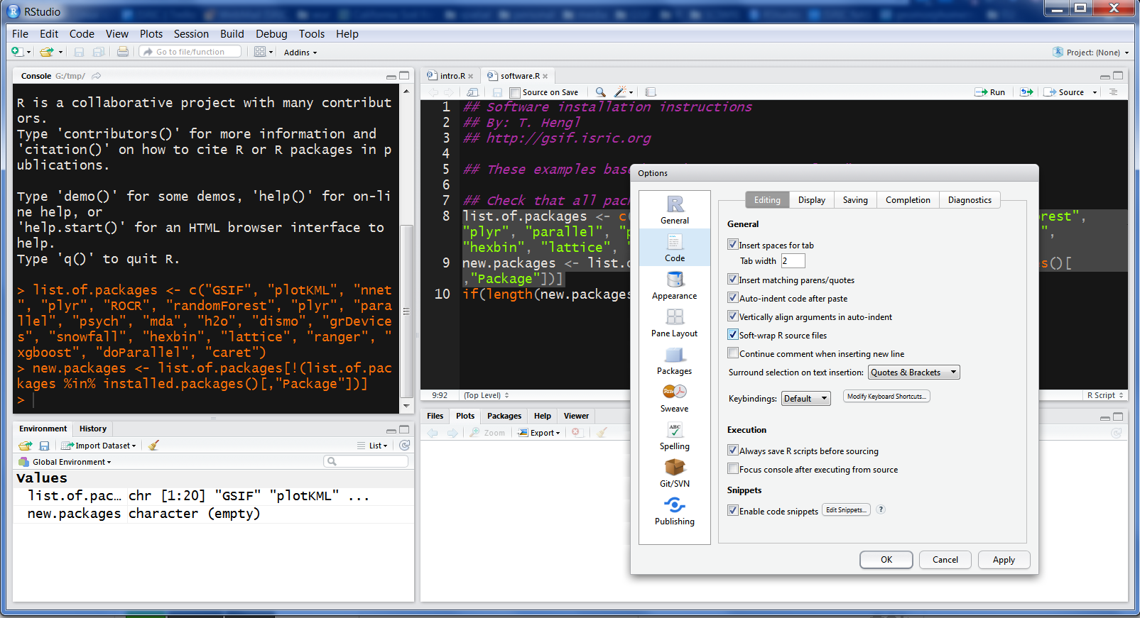
Figure 2.4: RStudio is a commonly used R editor written in C++.
To install all required R packages used in this tutorial at once, you can use:
ls <- c("reshape", "Hmisc", "rgdal", "raster", "sf", "GSIF", "plotKML",
        "nnet", "plyr", "ROCR", "randomForest", "quantregForest",
        "psych", "mda", "h2o", "h2oEnsemble", "dismo", "grDevices",
        "snowfall", "hexbin", "lattice", "ranger",
        "soiltexture", "aqp", "colorspace", "Cubist",
        "randomForestSRC", "ggRandomForests", "scales",
        "xgboost", "parallel", "doParallel", "caret",
        "gam", "glmnet", "matrixStats", "SuperLearner",
        "quantregForest", "intamap", "fasterize", "viridis")
new.packages <- ls[!(ls %in% installed.packages()[,"Package"])]
if(length(new.packages)) install.packages(new.packages)
This will basically check if any package is installed already, then install it only if it is missing. You can put this line at the top of each R script that you share so that anybody using that script will automatically obtain all required packages.
Note that the h2o package requires Java libraries, so you will also have to install Java by using e.g.:
sudo add-apt-repository ppa:webupd8team/java
sudo apt-get update
sudo apt-get install oracle-java8-installer
java -version
2.6 plotKML and GSIF packages
Many examples in this tutorial rely on the top 5 most commonly used packages for spatial data: (1) sp and rgdal, (2) raster, (3) plotKML and (4) GSIF. To install the most up-to-date version of plotKML/GSIF, you can also use the R-Forge versions of the package:
if(!require(GSIF)){
  install.packages("GSIF", repos=c("http://R-Forge.R-project.org"),
                 type = "source", dependencies = TRUE)
}
#> Loading required package: GSIF
#> GSIF version 0.5-5 (2019-01-04)
#> URL: http://gsif.r-forge.r-project.org/
A copy of the most-up-to-date and stable versions of plotKML and GSIF is also available on github. To run only some specific function from the GSIF package you can do e.g.:
source_https <- function(url, ...) {
   # load package
   require(RCurl)
   # download:
   cat(getURL(url, followlocation = TRUE,
       cainfo = system.file("CurlSSL", "cacert.pem", package = "RCurl")),
       file = basename(url))
   source(basename(url))
}
source_https("https://raw.githubusercontent.com/cran/GSIF/master/R/OCSKGM.R")
To test if these packages work properly, create soil maps and visualize them in Google Earth by running the following lines of code (see also function: fit.gstatModel):
library(GSIF)
library(sp)
library(boot)
library(aqp)
#> This is aqp 1.17
#>
#> Attaching package: 'aqp'
#> The following object is masked from 'package:base':
#>
#>     union
library(plyr)
library(rpart)
library(splines)
library(gstat)
library(quantregForest)
#> Loading required package: randomForest
#> randomForest 4.6-14
#> Type rfNews() to see new features/changes/bug fixes.
#> Loading required package: RColorBrewer
library(plotKML)
#> plotKML version 0.5-9 (2019-01-04)
#> URL: http://plotkml.r-forge.r-project.org/
demo(meuse, echo=FALSE)
omm <- fit.gstatModel(meuse, om~dist+ffreq, meuse.grid, method="quantregForest")
#> Fitting a Quantile Regression Forest model...
#> Fitting a 2D variogram...
#> Saving an object of class 'gstatModel'...
om.rk <- predict(omm, meuse.grid)
#> Subsetting observations to fit the prediction domain in 2D...
#> Prediction error for 'randomForest' model estimated using the 'quantreg' package.
#> Generating predictions using the trend model (RK method)...
#> [using ordinary kriging]
#>
100% done
#> Running 5-fold cross validation using 'krige.cv'...
#> Creating an object of class "SpatialPredictions"
om.rk
#>   Variable           : om
#>   Minium value       : 1
#>   Maximum value      : 17
#>   Size               : 153
#>   Total area         : 4964800
#>   Total area (units) : square-m
#>   Resolution (x)     : 40
#>   Resolution (y)     : 40
#>   Resolution (units) : m
#>   Vgm model          : Exp
#>   Nugget (residual)  : 2.32
#>   Sill (residual)    : 4.76
#>   Range (residual)   : 2930
#>   RMSE (validation)  : 1.75
#>   Var explained      : 73.8%
#>   Effective bytes    : 1202
#>   Compression method : gzip
#plotKML(om.rk)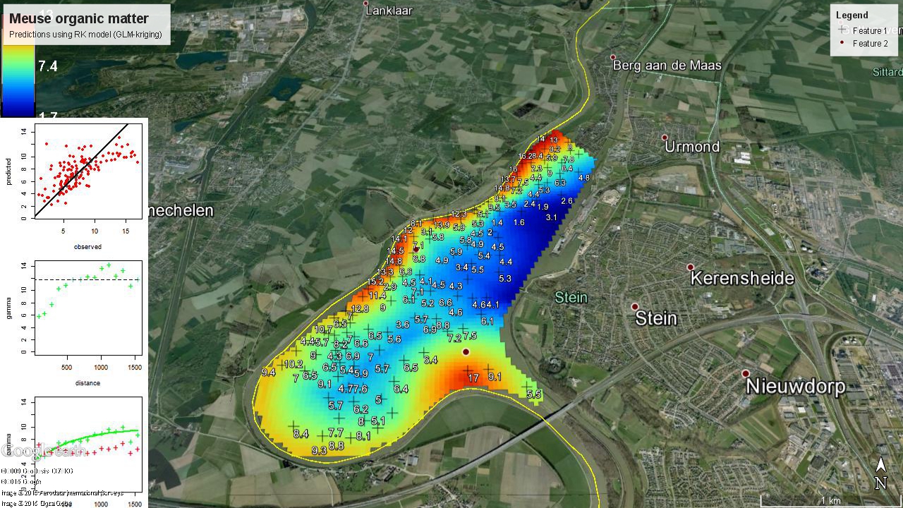
Figure 2.5: Example of a plotKML output for geostatistical model and prediction.
2.7 Connecting R and SAGA GIS
SAGA GIS provides comprehensive GIS geoprocessing software with over 600 functions.
SAGA GIS can not be installed from RStudio (it is not a package for R).
Instead, you need to install SAGA GIS using the installation instructions from the software homepage.
After you have installed SAGA GIS, you can send processes from
R to SAGA GIS by using the saga_cmd command line interface:
if(Sys.info()['sysname']=="Windows"){
  saga_cmd = "C:/Progra~1/SAGA-GIS/saga_cmd.exe"
} else {
  saga_cmd = "saga_cmd"
}
system(paste(saga_cmd, "-v"))
#> Warning in system(paste(saga_cmd, "-v")): error in running command
To use some SAGA GIS function you need to carefully follow the SAGA GIS command line arguments. For example,
library(plotKML)
library(rgdal)
#> rgdal: version: 1.3-6, (SVN revision 773)
#>  Geospatial Data Abstraction Library extensions to R successfully loaded
#>  Loaded GDAL runtime: GDAL 2.2.2, released 2017/09/15
#>  Path to GDAL shared files: /usr/share/gdal/2.2
#>  GDAL binary built with GEOS: TRUE
#>  Loaded PROJ.4 runtime: Rel. 4.8.0, 6 March 2012, [PJ_VERSION: 480]
#>  Path to PROJ.4 shared files: (autodetected)
#>  Linking to sp version: 1.3-1
library(raster)
#>
#> Attaching package: 'raster'
#> The following objects are masked from 'package:aqp':
#>
#>     metadata, metadata<-
data("eberg_grid")
gridded(eberg_grid) <- ~x+y
proj4string(eberg_grid) <- CRS("+init=epsg:31467")
writeGDAL(eberg_grid["DEMSRT6"], "./extdata/DEMSRT6.sdat", "SAGA")
system(paste(saga_cmd, 'ta_lighting 0 -ELEVATION "./extdata/DEMSRT6.sgrd"
             -SHADE "./extdata/hillshade.sgrd" -EXAGGERATION 2'))
#> Warning in system(paste(saga_cmd, "ta_lighting 0 -ELEVATION \"./extdata/
#> DEMSRT6.sgrd\" \n -SHADE \"./extdata/hillshade.sgrd\" -EXAGGERATION 2")):
#> error in running command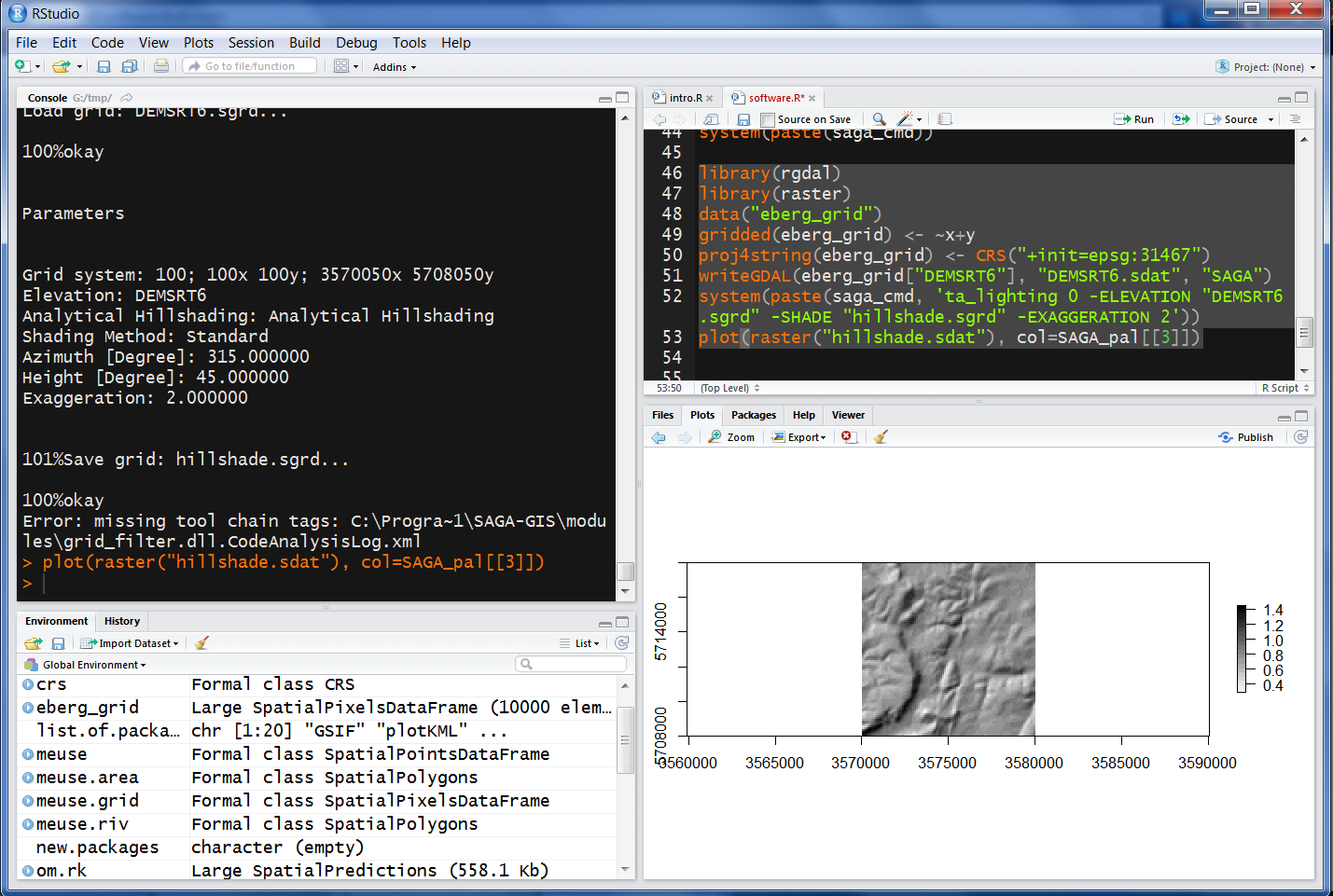
Figure 2.6: Deriving hillshading using SAGA GIS and then visualizing the result in R.
2.8 Connecting R and GDAL
GDAL is another very important software tool for handling spatial data (and especially for exchanging / converting spatial data). GDAL also needs to be installed separately (for Windows machines use e.g. “gdal-201-1800-x64-core.msi”) and then can be called from command line:
if(.Platform$OS.type == "windows"){
  gdal.dir <- shortPathName("C:/Program files/GDAL")
  gdal_translate <- paste0(gdal.dir, "/gdal_translate.exe")
  gdalwarp <- paste0(gdal.dir, "/gdalwarp.exe")
} else {
  gdal_translate = "gdal_translate"
  gdalwarp = "gdalwarp"
}
system(paste(gdalwarp, "--help"))
#> Warning in system(paste(gdalwarp, "--help")): error in running command
We can use GDAL to reproject the grid from the previous example:
system(paste('gdalwarp ./extdata/DEMSRT6.sdat ./extdata/DEMSRT6_ll.tif',
             '-t_srs \"+proj=longlat +datum=WGS84\"'))
#> Warning in system(paste("gdalwarp ./extdata/DEMSRT6.sdat ./extdata/
#> DEMSRT6_ll.tif", : error in running command
library(raster)
plot(raster("./extdata/DEMSRT6_ll.tif"))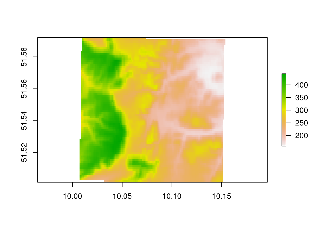
Figure 2.7: Ebergotzen DEM reprojected in geographical coordinates.
The following books are highly recommended for improving programming skills in R and specially for the purpose of geographical computing:
Bivand, R., Pebesma, E., Rubio, V., (2013) Applied Spatial Data Analysis with R. Use R Series, Springer, Heidelberg, 2nd Ed. 400 pages.
Lovelace, R., Nowosad, J., Muenchow, J., (2018) Geocomputation with R. R Series, CRC Press, 338 pages.
References
Conrad, O., B. Bechtel, M. Bock, H. Dietrich, E. Fischer, L. Gerlitz, J. Wehberg, V. Wichmann, and J. Böhner. 2015. “System for Automated Geoscientific Analyses (Saga) V. 2.1.4.” Geoscientific Model Development 8 (7). Copernicus GmbH:1991–2007. https://doi.org/10.5194/gmd-8-1991-2015.
Hijmans, Robert J., and Jacob van Etten. 2017. Raster: Geographic Data Analysis and Modeling. http://CRAN.R-project.org/package=raster.
Pebesma, Edzer J, and Roger S Bivand. 2005. “Classes and Methods for Spatial Data in R.” R News 5 (2):9–13.
Mitchell, T., and GDAL Developers. 2014. Geospatial Power Tools: GDAL Raster & Vector Commands. Locate Press.
Hengl, T., P. Roudier, D. Beaudette, and E. Pebesma. 2015. “PlotKML: Scientific Visualization of Spatio-Temporal Data.” Journal of Statistical Software 63 (5):1–25. http://www.jstatsoft.org/v63/i05/.
Lindsay, John B. 2016. “Whitebox GAT: A case study in geomorphometric analysis.” Computers & Geosciences 95. Elsevier:75–84.