6 Machine Learning Algorithms for soil mapping
Edited by: T. Hengl
6.1 Spatial prediction of soil properties and classes using MLA’s
This chapter reviews some common Machine learning algorithms (MLA’s) that have demonstrated potential for soil mapping projects i.e. for generating spatial predictions (Brungard et al. 2015; Heung et al. 2016; Thorsten Behrens et al. 2018). In this tutorial we especially focus on using tree-based algorithms such as random forest, gradient boosting and Cubist. For a more in-depth overview of machine learning algorithms used in statistics refer to the CRAN Task View on Machine Learning & Statistical Learning. As a gentle introduction to Machine and Statistical Learning we recommend:
Irizarry, R.A., (2018) Introduction to Data Science: Data Analysis and Prediction Algorithms with R. HarvardX Data Science Series.
Kuhn, M., Johnson, K. (2013) Applied Predictive Modeling. Springer Science, ISBN: 9781461468493, 600 pages.
Molnar, C. (2019) Interpretable Machine Learning: A Guide for Making Black Box Models Explainable, Leanpub, 251 pages.
Some other examples of how MLA’s can be used to fit Pedo-Transfer-Functions can be found in section 3.8.
6.1.1 Loading the packages and data
We use the following packages:
library(plotKML)
#> plotKML version 0.5-9 (2019-01-04)
#> URL: http://plotkml.r-forge.r-project.org/
library(sp)
library(randomForest)
#> randomForest 4.6-14
#> Type rfNews() to see new features/changes/bug fixes.
library(nnet)
library(e1071)
library(GSIF)
#> GSIF version 0.5-5 (2019-01-04)
#> URL: http://gsif.r-forge.r-project.org/
library(plyr)
library(raster)
#>
#> Attaching package: 'raster'
#> The following object is masked from 'package:e1071':
#>
#>     interpolate
library(caret)
#> Loading required package: lattice
#> Loading required package: ggplot2
#>
#> Attaching package: 'ggplot2'
#> The following object is masked from 'package:randomForest':
#>
#>     margin
library(Cubist)
library(GSIF)
library(xgboost)
library(viridis)
#> Loading required package: viridisLite
Next, we load the (Ebergotzen) data set which consists of point data collected using a soil auger and a stack of rasters containing all covariates:
library(plotKML)
data(eberg)
data(eberg_grid)
coordinates(eberg) <- ~X+Y
proj4string(eberg) <- CRS("+init=epsg:31467")
gridded(eberg_grid) <- ~x+y
proj4string(eberg_grid) <- CRS("+init=epsg:31467")
The covariates are then converted to principal components to reduce covariance and dimensionality:
eberg_spc <- spc(eberg_grid, ~ PRMGEO6+DEMSRT6+TWISRT6+TIRAST6)
#> Converting PRMGEO6 to indicators...
#> Converting covariates to principal components...
eberg_grid@data <- cbind(eberg_grid@data, eberg_spc@predicted@data)
All further analysis is run using the so-called regression matrix (matrix produced using the overlay of points and grids), which contains values of the target variable and all covariates for all training points:
ov <- over(eberg, eberg_grid)
m <- cbind(ov, eberg@data)
dim(m)
#> [1] 3670   44
In this case the regression matrix consists of 3670 observations and has 44 columns.
6.1.2 Spatial prediction of soil classes using MLA’s
In the first example, we focus on mapping soil types using the auger point data. First, we need to filter out some classes that do not occur frequently enough to support statistical modelling. As a rule of thumb, a class to be modelled should have at least 5 observations:
xg <- summary(m$TAXGRSC, maxsum=(1+length(levels(m$TAXGRSC))))
str(xg)
#>  Named int [1:14] 71 790 86 1 186 1 704 215 252 487 ...
#>  - attr(*, "names")= chr [1:14] "Auenboden" "Braunerde" "Gley" "HMoor" ...
selg.levs <- attr(xg, "names")[xg > 5]
attr(xg, "names")[xg <= 5]
#> [1] "HMoor" "Moor"
this shows that two classes probably have too few observations and should be excluded from further modeling:
m$soiltype <- m$TAXGRSC
m$soiltype[which(!m$TAXGRSC %in% selg.levs)] <- NA
m$soiltype <- droplevels(m$soiltype)
str(summary(m$soiltype, maxsum=length(levels(m$soiltype))))
#>  Named int [1:11] 790 704 487 376 252 215 186 86 71 43 ...
#>  - attr(*, "names")= chr [1:11] "Braunerde" "Parabraunerde" "Pseudogley" "Regosol" ...
We can also remove all points that contain missing values for any combination of covariates and target variable:
m <- m[complete.cases(m[,1:(ncol(eberg_grid)+2)]),]
m$soiltype <- as.factor(m$soiltype)
summary(m$soiltype)
#>     Auenboden     Braunerde          Gley    Kolluvisol Parabraunerde
#>            48           669            68           138           513
#>  Pararendzina       Pelosol    Pseudogley        Ranker       Regosol
#>           176           177           411            17           313
#>      Rendzina
#>            22
We can now test fitting a MLA i.e. a random forest model using four covariate layers (parent material map, elevation, TWI and ASTER thermal band):
## subset to speed-up:
s <- sample.int(nrow(m), 500)
TAXGRSC.rf <- randomForest(x=m[-s,paste0("PC",1:10)], y=m$soiltype[-s],
                           xtest=m[s,paste0("PC",1:10)], ytest=m$soiltype[s])
## accuracy:
TAXGRSC.rf$test$confusion[,"class.error"]
#>     Auenboden     Braunerde          Gley    Kolluvisol Parabraunerde
#>         0.750         0.479         0.846         0.652         0.571
#>  Pararendzina       Pelosol    Pseudogley        Ranker       Regosol
#>         0.571         0.696         0.690         1.000         0.625
#>      Rendzina
#>         0.500
Note that, by specifying xtest and ytest, we run both model fitting and cross-validation with 500 excluded points. The results show relatively high prediction error of about 60% i.e. relative classification accuracy of about 40%.
We can also test some other MLA’s that are suited for this data — multinom from the nnet package, and svm (Support Vector Machine) from the e1071 package:
TAXGRSC.rf <- randomForest(x=m[,paste0("PC",1:10)], y=m$soiltype)
fm <- as.formula(paste("soiltype~", paste(paste0("PC",1:10), collapse="+")))
TAXGRSC.mn <- nnet::multinom(fm, m)
#> # weights:  132 (110 variable)
#> initial  value 6119.428736
#> iter  10 value 4161.338634
#> iter  20 value 4118.296050
#> iter  30 value 4054.454486
#> iter  40 value 4020.653949
#> iter  50 value 3995.113270
#> iter  60 value 3980.172669
#> iter  70 value 3975.188371
#> iter  80 value 3973.743572
#> iter  90 value 3973.073564
#> iter 100 value 3973.064186
#> final  value 3973.064186
#> stopped after 100 iterations
TAXGRSC.svm <- e1071::svm(fm, m, probability=TRUE, cross=5)
TAXGRSC.svm$tot.accuracy
#> [1] 40.1
This produces about the same accuracy levels as for random forest. Because all three methods produce comparable accuracy, we can also merge predictions by calculating a simple average:
probs1 <- predict(TAXGRSC.mn, eberg_grid@data, type="probs", na.action = na.pass)
probs2 <- predict(TAXGRSC.rf, eberg_grid@data, type="prob", na.action = na.pass)
probs3 <- attr(predict(TAXGRSC.svm, eberg_grid@data,
                       probability=TRUE, na.action = na.pass), "probabilities")
derive average prediction:
leg <- levels(m$soiltype)
lt <- list(probs1[,leg], probs2[,leg], probs3[,leg])
probs <- Reduce("+", lt) / length(lt)
## copy and make new raster object:
eberg_soiltype <- eberg_grid
eberg_soiltype@data <- data.frame(probs)
Check that all predictions sum up to 100%:
ch <- rowSums(eberg_soiltype@data)
summary(ch)
#>    Min. 1st Qu.  Median    Mean 3rd Qu.    Max.
#>       1       1       1       1       1       1
To plot the result we can use the raster package (Fig. 6.1):
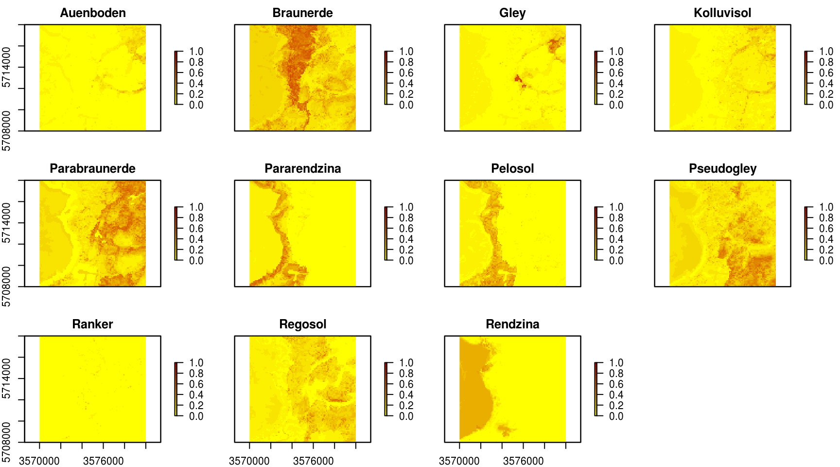
Figure 6.1: Predicted soil types for the Ebergotzen case study.
By using the produced predictions we can further derive Confusion Index (to map thematic uncertainty) and see if some classes should be aggregated. We can also generate a factor-type map by selecting the most probable class for each pixel, by using e.g.:
eberg_soiltype$cl <- as.factor(apply(eberg_soiltype@data,1,which.max))
levels(eberg_soiltype$cl) = attr(probs, "dimnames")[[2]][as.integer(levels(eberg_soiltype$cl))]
summary(eberg_soiltype$cl)
#>     Auenboden     Braunerde          Gley    Kolluvisol Parabraunerde
#>            36          2286           146            68          2253
#>  Pararendzina       Pelosol    Pseudogley       Regosol      Rendzina
#>           821           439          1310           317          2324
6.1.3 Modelling numeric soil properties using h2o
Random forest is suited for both classification and regression problems (it is one of the most popular MLA’s for soil mapping). Consequently, we can use it also for modelling numeric soil properties i.e. to fit models and generate predictions. However, because the randomForest package in R is not suited for large data sets, we can also use some parallelized version of random forest (or more scalable) i.e. the one implemented in the h2o package (Richter et al. 2015). h2o is a Java-based implementation, therefore installing the package requires Java libraries (size of package is about 80MB so it might take some to download and install) and all computing is, in principle, run outside of R i.e. within the JVM (Java Virtual Machine).
In the following example we look at mapping sand content for the upper horizons. To initiate h2o we run:
library(h2o)
localH2O = h2o.init(startH2O=TRUE)
#>  Connection successful!
#>
#> R is connected to the H2O cluster:
#>     H2O cluster uptime:         23 minutes 43 seconds
#>     H2O cluster timezone:       UTC
#>     H2O data parsing timezone:  UTC
#>     H2O cluster version:        3.22.1.1
#>     H2O cluster version age:    2 months and 17 days
#>     H2O cluster name:           H2O_started_from_R_travis_lqb476
#>     H2O cluster total nodes:    1
#>     H2O cluster total memory:   1.40 GB
#>     H2O cluster total cores:    2
#>     H2O cluster allowed cores:  2
#>     H2O cluster healthy:        TRUE
#>     H2O Connection ip:          localhost
#>     H2O Connection port:        54321
#>     H2O Connection proxy:       NA
#>     H2O Internal Security:      FALSE
#>     H2O API Extensions:         XGBoost, Algos, AutoML, Core V3, Core V4
#>     R Version:                  R version 3.5.2 (2017-01-27)
This shows that multiple cores will be used for computing (to control the number of cores you can use the nthreads argument). Next, we need to prepare the regression matrix and prediction locations using the as.h2o function so that they are visible to h2o:
eberg.hex <- as.h2o(m, destination_frame = "eberg.hex")
eberg.grid <- as.h2o(eberg_grid@data, destination_frame = "eberg.grid")
We can now fit a random forest model by using all the computing power available to us:
RF.m <- h2o.randomForest(y = which(names(m)=="SNDMHT_A"),
                        x = which(names(m) %in% paste0("PC",1:10)),
                        training_frame = eberg.hex, ntree = 50)
RF.m
#> Model Details:
#> ==============
#>
#> H2ORegressionModel: drf
#> Model ID:  DRF_model_R_1552840950825_21
#> Model Summary:
#>   number_of_trees number_of_internal_trees model_size_in_bytes min_depth
#> 1              50                       50              647929        20
#>   max_depth mean_depth min_leaves max_leaves mean_leaves
#> 1        20   20.00000        969       1083  1027.90000
#>
#>
#> H2ORegressionMetrics: drf
#> ** Reported on training data. **
#> ** Metrics reported on Out-Of-Bag training samples **
#>
#> MSE:  216
#> RMSE:  14.7
#> MAE:  10
#> RMSLE:  0.426
#> Mean Residual Deviance :  216
This shows that the model fitting R-square is about 50%. This is also indicated by the predicted vs observed plot:
library(scales)
#>
#> Attaching package: 'scales'
#> The following object is masked from 'package:viridis':
#>
#>     viridis_pal
library(lattice)
SDN.pred <- as.data.frame(h2o.predict(RF.m, eberg.hex, na.action=na.pass))$predict
plt1 <- xyplot(m$SNDMHT_A ~ SDN.pred, asp=1,
               par.settings=list(
                 plot.symbol = list(col=scales::alpha("black", 0.6),
                 fill=scales::alpha("red", 0.6), pch=21, cex=0.8)),
                 ylab="measured", xlab="predicted (machine learning)")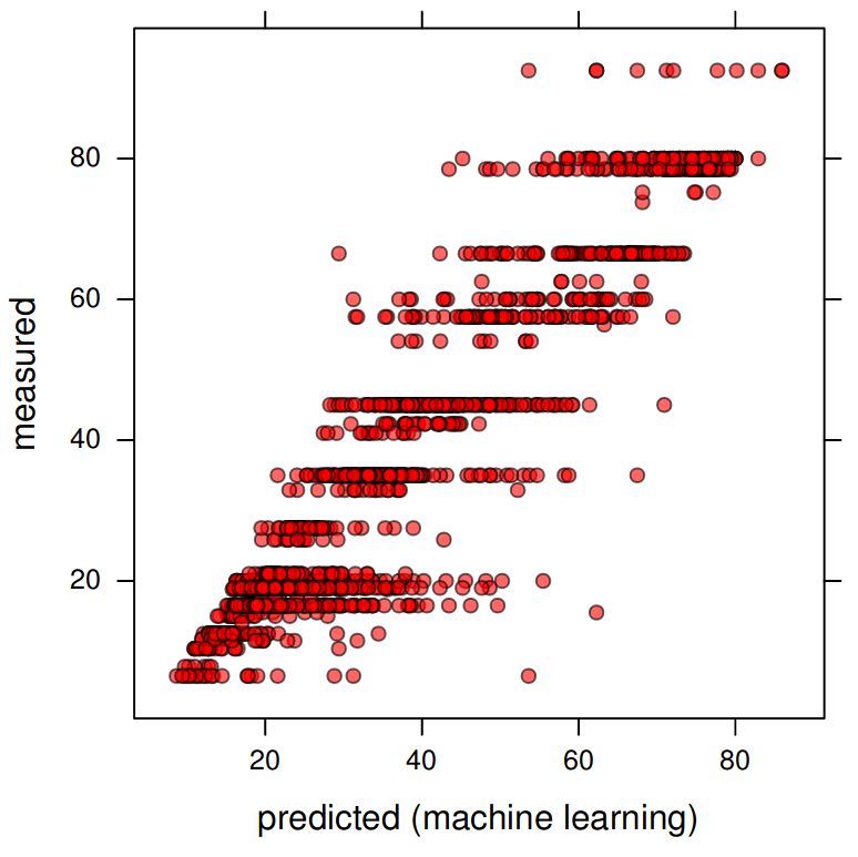
Figure 6.2: Measured vs predicted sand content based on the Random Forest model.
To produce a map based on these predictions we use:
eberg_grid$RFx <- as.data.frame(h2o.predict(RF.m, eberg.grid, na.action=na.pass))$predict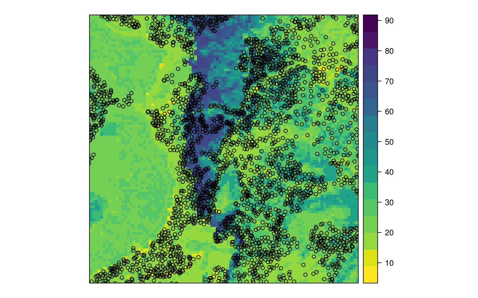
Figure 6.3: Predicted sand content based on random forest.
h2o has another MLA of interest for soil mapping called deep learning (a feed-forward multilayer artificial neural network). Fitting the model is equivalent to using random forest:
DL.m <- h2o.deeplearning(y = which(names(m)=="SNDMHT_A"),
                         x = which(names(m) %in% paste0("PC",1:10)),
                         training_frame = eberg.hex)
DL.m
#> Model Details:
#> ==============
#>
#> H2ORegressionModel: deeplearning
#> Model ID:  DeepLearning_model_R_1552840950825_22
#> Status of Neuron Layers: predicting SNDMHT_A, regression, gaussian distribution, Quadratic loss, 42,601 weights/biases, 508.3 KB, 25,520 training samples, mini-batch size 1
#>   layer units      type dropout       l1       l2 mean_rate rate_rms
#> 1     1    10     Input  0.00 %       NA       NA        NA       NA
#> 2     2   200 Rectifier  0.00 % 0.000000 0.000000  0.014556 0.009009
#> 3     3   200 Rectifier  0.00 % 0.000000 0.000000  0.138473 0.184169
#> 4     4     1    Linear      NA 0.000000 0.000000  0.001368 0.000909
#>   momentum mean_weight weight_rms mean_bias bias_rms
#> 1       NA          NA         NA        NA       NA
#> 2 0.000000   -0.001292   0.102565  0.352788 0.067968
#> 3 0.000000   -0.018166   0.070974  0.953664 0.021549
#> 4 0.000000    0.000102   0.046915  0.134803 0.000000
#>
#>
#> H2ORegressionMetrics: deeplearning
#> ** Reported on training data. **
#> ** Metrics reported on full training frame **
#>
#> MSE:  283
#> RMSE:  16.8
#> MAE:  12.7
#> RMSLE:  0.518
#> Mean Residual Deviance :  283
Which delivers performance comparable to the random forest model. The output prediction map does show somewhat different patterns than the random forest predictions (compare Fig. 6.3 and Fig. 6.4).
## predictions:
eberg_grid$DLx <- as.data.frame(h2o.predict(DL.m, eberg.grid, na.action=na.pass))$predict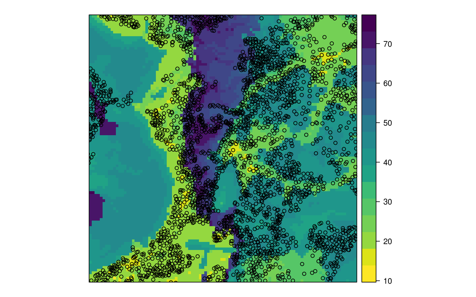
Figure 6.4: Predicted sand content based on deep learning.
Which of the two methods should we use? Since they both have comparable performance, the most logical option is to generate ensemble (merged) predictions i.e. to produce a map that shows patterns averaged between the two methods (note: many sophisticated MLA such as random forest, neural nets, SVM and similar will often produce comparable results i.e. they are often equally applicable and there is no clear winner). We can use weighted average i.e. R-square as a simple approach to produce merged predictions:
rf.R2 <- RF.m@model$training_metrics@metrics$r2
dl.R2 <- DL.m@model$training_metrics@metrics$r2
eberg_grid$SNDMHT_A <- rowSums(cbind(eberg_grid$RFx*rf.R2,
                         eberg_grid$DLx*dl.R2), na.rm=TRUE)/(rf.R2+dl.R2)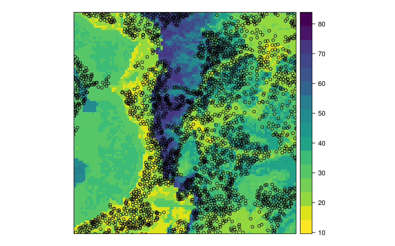
Figure 6.5: Predicted sand content based on ensemble predictions.
Indeed, the output map now shows patterns of both methods and is more likely slightly more accurate than any of the individual MLA’s (Sollich and Krogh 1996).
6.1.4 Spatial prediction of 3D (numeric) variables
In the final exercise, we look at another two ML-based packages that are also of interest for soil mapping projects — cubist (Kuhn et al. 2012; Kuhn and Johnson 2013) and xgboost (Chen and Guestrin 2016). The object is now to fit models and predict continuous soil properties in 3D. To fine-tune some of the models we will also use the caret package, which is highly recommended for optimizing model fitting and cross-validation. Read more about how to derive soil organic carbon stock using 3D soil mapping in section 7.7.
We will use another soil mapping data set from Australia called “Edgeroi”, which is described in detail in Malone et al. (2009). We can load the profile data and covariates by using:
data(edgeroi)
edgeroi.sp <- edgeroi$sites
coordinates(edgeroi.sp) <- ~ LONGDA94 + LATGDA94
proj4string(edgeroi.sp) <- CRS("+proj=longlat +ellps=GRS80 +towgs84=0,0,0,0,0,0,0 +no_defs")
edgeroi.sp <- spTransform(edgeroi.sp, CRS("+init=epsg:28355"))
load("extdata/edgeroi.grids.rda")
gridded(edgeroi.grids) <- ~x+y
proj4string(edgeroi.grids) <- CRS("+init=epsg:28355")
Here we are interested in modelling soil organic carbon content in g/kg for different depths. We again start by producing the regression matrix:
ov2 <- over(edgeroi.sp, edgeroi.grids)
ov2$SOURCEID <- edgeroi.sp$SOURCEID
str(ov2)
#> 'data.frame':    359 obs. of  7 variables:
#>  $ DEMSRT5 : num  208 199 203 202 195 201 198 210 190 195 ...
#>  $ TWISRT5 : num  19.8 19.9 19.7 19.3 19.3 19.7 19.5 19.6 19.6 19.2 ...
#>  $ PMTGEO5 : Factor w/ 7 levels "Qd","Qrs","Qrt/Jp",..: 2 2 2 2 2 2 2 2 2 2 ...
#>  $ EV1MOD5 : num  -0.08 2.41 2.62 -0.39 -0.78 -0.75 1.14 5.16 -0.48 -0.84 ...
#>  $ EV2MOD5 : num  -2.47 -2.84 -2.43 5.2 1.27 -4.96 1.62 1.33 -2.66 1.01 ...
#>  $ EV3MOD5 : num  -1.59 -0.31 1.43 1.96 -0.44 2.47 -5.74 -6.78 2.29 -1.59 ...
#>  $ SOURCEID: Factor w/ 359 levels "199_CAN_CP111_1",..: 1 2 3 4 5 6 7 8 9 10 ...
Because we will run 3D modelling, we also need to add depth of horizons. We use a small function to assign depth values as the center depth of each horizon (as shown in figure below). Because we know where the horizons start and stop, we can copy the values of target variables two times so that the model knows at which depths values of properties change.
## Convert soil horizon data to x,y,d regression matrix for 3D modeling:
hor2xyd <- function(x, U="UHDICM", L="LHDICM", treshold.T=15){
  x$DEPTH <- x[,U] + (x[,L] - x[,U])/2
  x$THICK <- x[,L] - x[,U]
  sel <- x$THICK < treshold.T
  ## begin and end of the horizon:
  x1 <- x[!sel,]; x1$DEPTH = x1[,L]
  x2 <- x[!sel,]; x2$DEPTH = x1[,U]
  y <- do.call(rbind, list(x, x1, x2))
  return(y)
}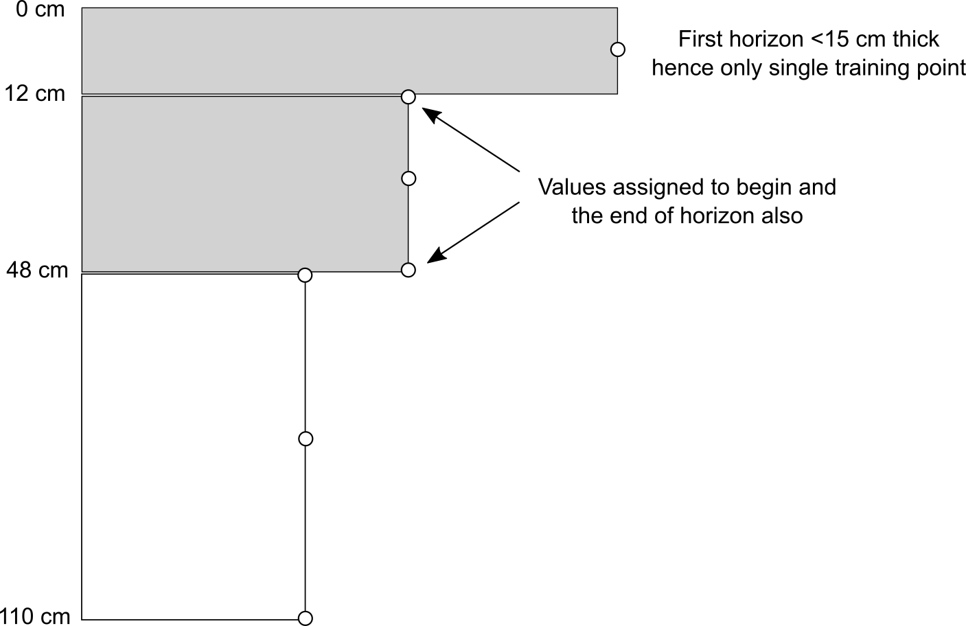
Figure 6.6: Training points assigned to a soil profile with 3 horizons. Using the function from above, we assign a total of 7 training points i.e. about 2 times more training points than there are horizons.
h2 <- hor2xyd(edgeroi$horizons)
## regression matrix:
m2 <- plyr::join_all(dfs = list(edgeroi$sites, h2, ov2))
#> Joining by: SOURCEID
#> Joining by: SOURCEID
## spatial prediction model:
formulaStringP2 <- ORCDRC ~ DEMSRT5+TWISRT5+PMTGEO5+
                            EV1MOD5+EV2MOD5+EV3MOD5+DEPTH
mP2 <- m2[complete.cases(m2[,all.vars(formulaStringP2)]),]
Note that DEPTH is used as a covariate, which makes this model 3D as one can predict anywhere in 3D space. To improve random forest modelling, we use the caret package that tries to identify also the optimal mtry parameter i.e. based on the cross-validation performance:
library(caret)
ctrl <- trainControl(method="repeatedcv", number=5, repeats=1)
sel <- sample.int(nrow(mP2), 500)
tr.ORCDRC.rf <- train(formulaStringP2, data = mP2[sel,],
                      method = "rf", trControl = ctrl, tuneLength = 3)
tr.ORCDRC.rf
#> Random Forest
#>
#> 500 samples
#>   7 predictor
#>
#> No pre-processing
#> Resampling: Cross-Validated (5 fold, repeated 1 times)
#> Summary of sample sizes: 400, 400, 400, 401, 399
#> Resampling results across tuning parameters:
#>
#>   mtry  RMSE  Rsquared  MAE
#>    2    3.58  0.580     2.41
#>    7    3.14  0.630     2.04
#>   12    3.21  0.609     2.06
#>
#> RMSE was used to select the optimal model using the smallest value.
#> The final value used for the model was mtry = 7.
In this case, mtry = 12 seems to achieve the best performance. Note that we sub-set the initial matrix to speed up fine-tuning of the parameters (otherwise the computing time could easily become too great). Next, we can fit the final model by using all data (this time we also turn cross-validation off):
ORCDRC.rf <- train(formulaStringP2, data=mP2,
                   method = "rf", tuneGrid=data.frame(mtry=7),
                   trControl=trainControl(method="none"))
w1 <- 100*max(tr.ORCDRC.rf$results$Rsquared)
The variable importance plot indicates that DEPTH is by far the most important predictor:
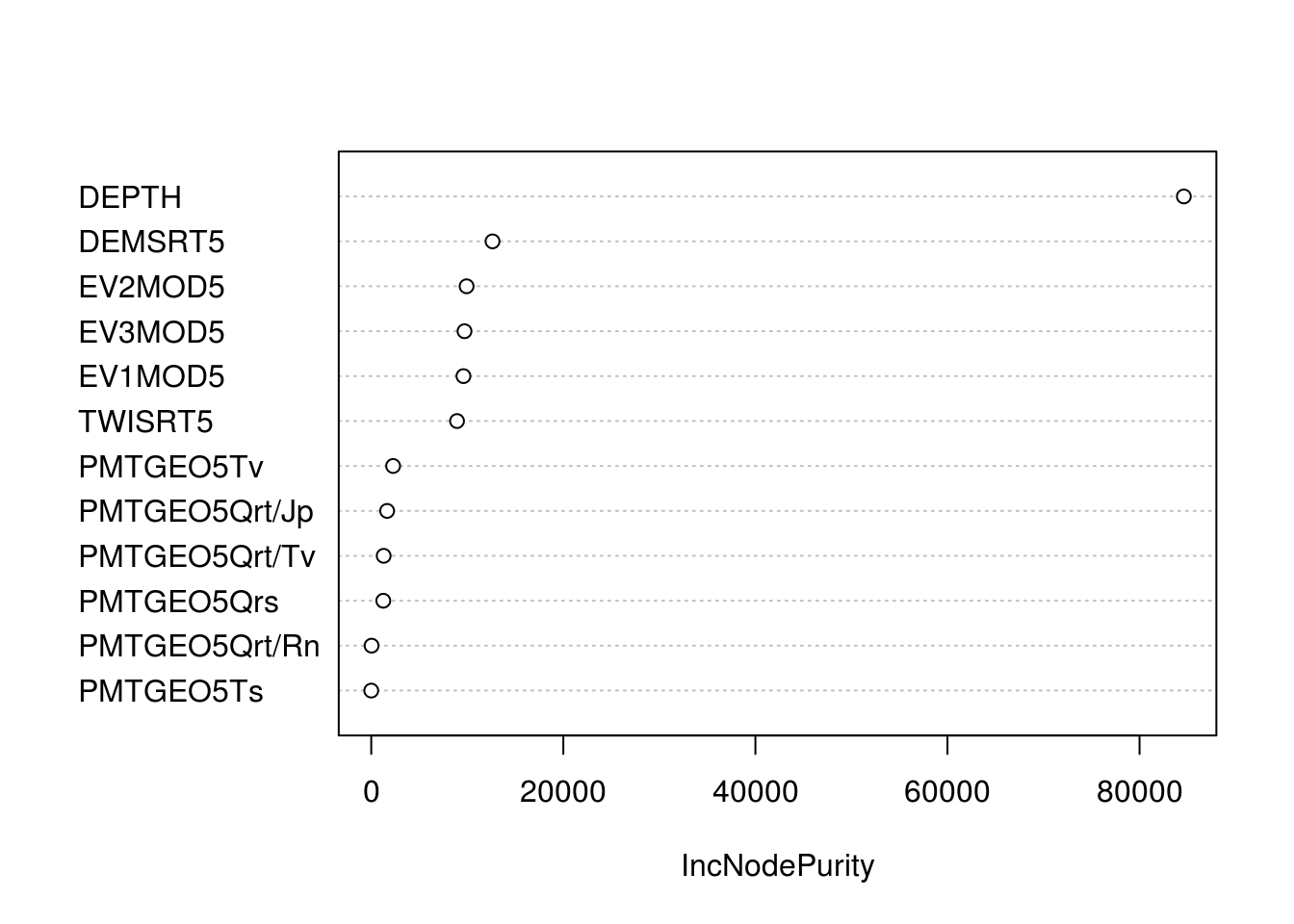
Figure 6.7: Variable importance plot for predicting soil organic carbon content (ORC) in 3D.
We can also try fitting models using the xgboost package and the cubist packages:
tr.ORCDRC.cb <- train(formulaStringP2, data=mP2[sel,],
                      method = "cubist", trControl = ctrl, tuneLength = 3)
ORCDRC.cb <- train(formulaStringP2, data=mP2,
                   method = "cubist",
                   tuneGrid=data.frame(committees = 1, neighbors = 0),
                   trControl=trainControl(method="none"))
w2 <- 100*max(tr.ORCDRC.cb$results$Rsquared)
## "XGBoost" package:
ORCDRC.gb <- train(formulaStringP2, data=mP2, method = "xgbTree", trControl=ctrl)
w3 <- 100*max(ORCDRC.gb$results$Rsquared)
c(w1, w2, w3)
#> [1] 63.0 65.9 66.6
At the end of the statistical modelling process, we can merge the predictions by using the CV R-square estimates:
edgeroi.grids$DEPTH <- 2.5
edgeroi.grids$Random_forest <- predict(ORCDRC.rf, edgeroi.grids@data,
                                       na.action = na.pass)
edgeroi.grids$Cubist <- predict(ORCDRC.cb, edgeroi.grids@data, na.action = na.pass)
edgeroi.grids$XGBoost <- predict(ORCDRC.gb, edgeroi.grids@data, na.action = na.pass)
edgeroi.grids$ORCDRC_5cm <- (edgeroi.grids$Random_forest*w1 +
                               edgeroi.grids$Cubist*w2 +
                               edgeroi.grids$XGBoost*w3)/(w1+w2+w3)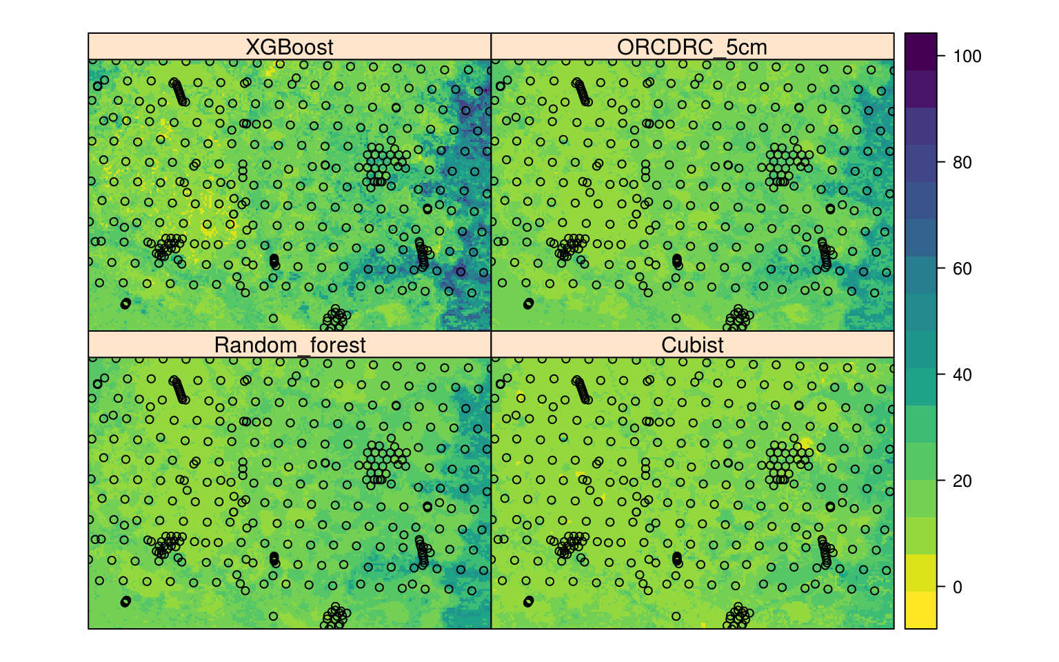
Figure 6.8: Comparison of three MLA’s and the final ensemble prediction (ORCDRC 5cm) of soil organic carbon content for 2.5 cm depth.
The final plot shows that xgboost possibly over-predicts and that cubist possibly under-predicts values of ORCDRC, while random forest is somewhere in-between the two. Again, merged predictions are probably the safest option considering that all three MLA’s have similar measures of performance.
We can quickly test the overall performance using a script on github prepared for testing performance of merged predictions:
source_https <- function(url, ...) {
  require(RCurl)
  if(!file.exists(paste0("R/", basename(url)))){
    cat(getURL(url, followlocation = TRUE,
               cainfo = system.file("CurlSSL", "cacert.pem", package = "RCurl")),
        file = paste0("R/", basename(url)))
  }
  source(paste0("R/", basename(url)))
}
wdir = "https://raw.githubusercontent.com/ISRICWorldSoil/SoilGrids250m/"
source_https(paste0(wdir, "master/grids/cv/cv_functions.R"))
#> Loading required package: RCurl
#> Loading required package: bitops
We can hence run 5-fold cross validation:
mP2$SOURCEID = paste(mP2$SOURCEID)
test.ORC <- cv_numeric(formulaStringP2, rmatrix=mP2,
                       nfold=5, idcol="SOURCEID", Log=TRUE)
#> Running 5-fold cross validation with model re-fitting method ranger ...
#> Subsetting observations by unique location
#> Loading required package: snowfall
#> Loading required package: snow
#> Warning in searchCommandline(parallel, cpus = cpus, type = type,
#> socketHosts = socketHosts, : Unknown option on commandline: --file
#> R Version:  R version 3.5.2 (2017-01-27)
#> snowfall 1.84-6.1 initialized (using snow 0.4-3): parallel execution on 2 CPUs.
#> Library plyr loaded.
#> Library plyr loaded in cluster.
#> Library ranger loaded.
#> Library ranger loaded in cluster.
#>
#> Attaching package: 'ranger'
#> The following object is masked from 'package:randomForest':
#>
#>     importance
#>
#> Stopping cluster
str(test.ORC)
#> List of 2
#>  $ CV_residuals:'data.frame':    4972 obs. of  4 variables:
#>   ..$ Observed : num [1:4972] 6.5 5.1 4.9 3.3 2.2 ...
#>   ..$ Predicted: num [1:4972] 12.22 7.5 6.47 4.98 3.2 ...
#>   ..$ SOURCEID : chr [1:4972] "399_EDGEROI_ed005_1" "399_EDGEROI_ed005_1" "399_EDGEROI_ed005_1" "399_EDGEROI_ed005_1" ...
#>   ..$ fold     : int [1:4972] 1 1 1 1 1 1 1 1 1 1 ...
#>  $ Summary     :'data.frame':    1 obs. of  6 variables:
#>   ..$ ME          : num -0.0971
#>   ..$ MAE         : num 2.18
#>   ..$ RMSE        : num 3.68
#>   ..$ R.squared   : num 0.557
#>   ..$ logRMSE     : num 0.492
#>   ..$ logR.squared: num 0.636
Which shows that the R-squared based on cross-validation is about 65% i.e. the average error of predicting soil organic carbon content using ensemble method is about \(\pm 4\) g/kg. The final observed-vs-predict plot shows that the model is unbiased and that the predictions generally match cross-validation points:
plt0 <- xyplot(test.ORC[[1]]$Observed ~ test.ORC[[1]]$Predicted, asp=1,
            par.settings = list(plot.symbol = list(col=scales::alpha("black", 0.6), fill=scales::alpha("red", 0.6), pch=21, cex=0.6)),
            scales = list(x=list(log=TRUE, equispaced.log=FALSE), y=list(log=TRUE, equispaced.log=FALSE)),
            ylab="measured", xlab="predicted (machine learning)")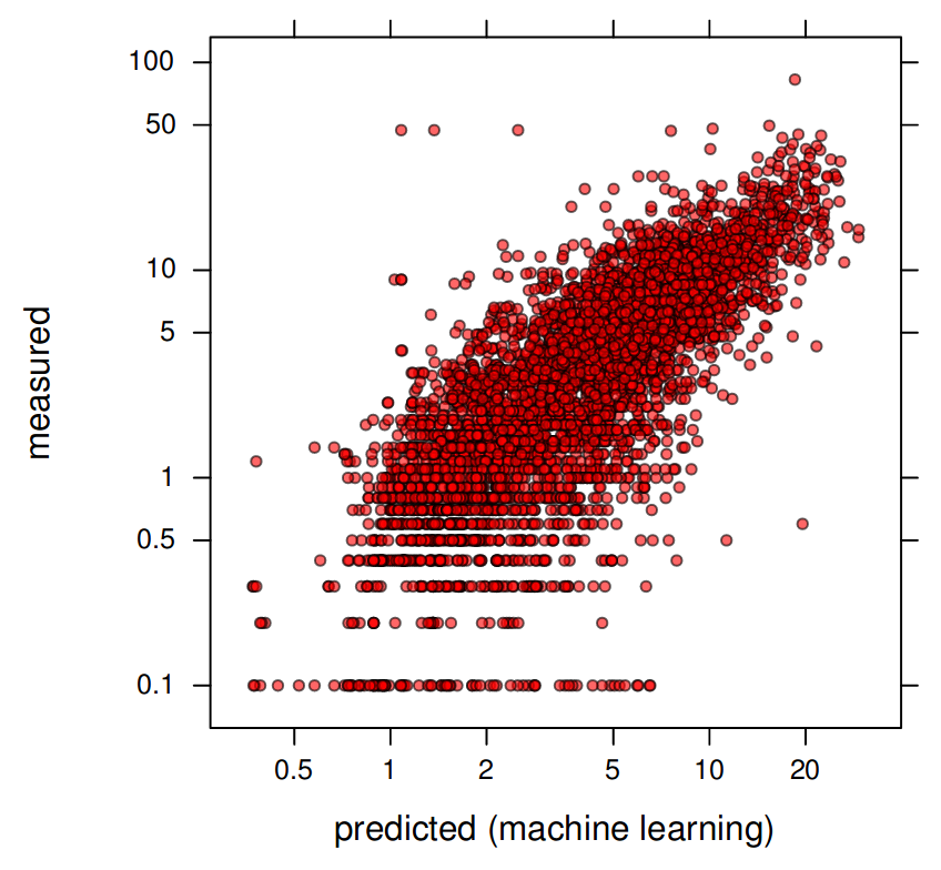
Figure 6.9: Predicted vs observed plot for soil organic carbon ML-based model (Edgeroi data set).
6.1.5 Ensemble predictions using h2oEnsemble
Ensemble models often outperform single models. There is certainly opportunity for increasing mapping accuracy by combining the power of 3–4 MLA’s. The h2o environment for ML offers automation of ensemble model fitting and predictions (LeDell 2015).
#> h2oEnsemble R package for H2O-3
#> Version: 0.2.1
#> Package created on 2017-08-02
we first specify all learners (MLA methods) of interest:
k.f = dismo::kfold(mP2, k=4)
summary(as.factor(k.f))
#>    1    2    3    4
#> 1243 1243 1243 1243
## split data into training and validation:
edgeroi_v.hex = as.h2o(mP2[k.f==1,], destination_frame = "eberg_v.hex")
edgeroi_t.hex = as.h2o(mP2[!k.f==1,], destination_frame = "eberg_t.hex")
learner <- c("h2o.randomForest.wrapper", "h2o.gbm.wrapper")
fit <- h2o.ensemble(x = which(names(m2) %in% all.vars(formulaStringP2)[-1]),
                    y = which(names(m2)=="ORCDRC"),
                    training_frame = edgeroi_t.hex, learner = learner,
                    cvControl = list(V = 5))
#> [1] "Cross-validating and training base learner 1: h2o.randomForest.wrapper"
#> Warning in h2o.randomForest(x = x, y = y, training_frame =
#> training_frame, : Argument offset_column is deprecated and has no use for
#> Random Forest.
#> [1] "Cross-validating and training base learner 2: h2o.gbm.wrapper"
#> [1] "Metalearning"
perf <- h2o.ensemble_performance(fit, newdata = edgeroi_v.hex)
#> Warning in doTryCatch(return(expr), name, parentenv, handler): Test/
#> Validation dataset is missing column 'fold_id': substituting in a column of
#> 0.0
#> Warning in doTryCatch(return(expr), name, parentenv, handler): Test/
#> Validation dataset is missing column 'fold_id': substituting in a column of
#> 0.0
perf
#>
#> Base learner performance, sorted by specified metric:
#>                    learner  MSE
#> 1 h2o.randomForest.wrapper 13.0
#> 2          h2o.gbm.wrapper 12.8
#>
#>
#> H2O Ensemble Performance on <newdata>:
#> ----------------
#> Family: gaussian
#>
#> Ensemble performance (MSE): 12.5019850661684
which shows that, in this specific case, the ensemble model is only slightly better than a single model. Note that we would need to repeat testing the ensemble modeling several times until we can be certain any actual actual gain in accuracy.
We can also test ensemble predictions using the cookfarm data set (Gasch et al. 2015). This data set consists of 183 profiles, each consisting of multiple soil horizons (1050 in total). To create a regression matrix we use:
data(cookfarm)
cookfarm.hor <- cookfarm$profiles
str(cookfarm.hor)
#> 'data.frame':    1050 obs. of  9 variables:
#>  $ SOURCEID: Factor w/ 369 levels "CAF001","CAF002",..: 3 3 3 3 3 5 5 5 5 5 ...
#>  $ Easting : num  493383 493383 493383 493383 493383 ...
#>  $ Northing: num  5180586 5180586 5180586 5180586 5180586 ...
#>  $ TAXSUSDA: Factor w/ 6 levels "Caldwell","Latah",..: 3 3 3 3 3 4 4 4 4 4 ...
#>  $ HZDUSD  : Factor w/ 67 levels "2R","A","A1",..: 12 2 7 35 36 12 2 16 43 44 ...
#>  $ UHDICM  : num  0 21 39 65 98 0 17 42 66 97 ...
#>  $ LHDICM  : num  21 39 65 98 153 17 42 66 97 153 ...
#>  $ BLD     : num  1.46 1.37 1.52 1.72 1.72 1.56 1.33 1.36 1.37 1.48 ...
#>  $ PHIHOX  : num  4.69 5.9 6.25 6.54 6.75 4.12 5.73 6.26 6.59 6.85 ...
cookfarm.hor$depth <- cookfarm.hor$UHDICM +
  (cookfarm.hor$LHDICM - cookfarm.hor$UHDICM)/2
sel.id <- !duplicated(cookfarm.hor$SOURCEID)
cookfarm.xy <- cookfarm.hor[sel.id,c("SOURCEID","Easting","Northing")]
str(cookfarm.xy)
#> 'data.frame':    183 obs. of  3 variables:
#>  $ SOURCEID: Factor w/ 369 levels "CAF001","CAF002",..: 3 5 7 9 11 13 15 17 19 21 ...
#>  $ Easting : num  493383 493447 493511 493575 493638 ...
#>  $ Northing: num  5180586 5180572 5180568 5180573 5180571 ...
coordinates(cookfarm.xy) <- ~ Easting + Northing
grid10m <- cookfarm$grids
coordinates(grid10m) <- ~ x + y
gridded(grid10m) = TRUE
ov.cf <- over(cookfarm.xy, grid10m)
rm.cookfarm <- plyr::join(cookfarm.hor, cbind(cookfarm.xy@data, ov.cf))
#> Joining by: SOURCEID
Here, we are interested in predicting soil pH in 3D, hence we will use a model of form:
fm.PHI <- PHIHOX~DEM+TWI+NDRE.M+Cook_fall_ECa+Cook_spr_ECa+depth
rc <- complete.cases(rm.cookfarm[,all.vars(fm.PHI)])
mP3 <- rm.cookfarm[rc,all.vars(fm.PHI)]
str(mP3)
#> 'data.frame':    997 obs. of  7 variables:
#>  $ PHIHOX       : num  4.69 5.9 6.25 6.54 6.75 4.12 5.73 6.26 6.59 6.85 ...
#>  $ DEM          : num  788 788 788 788 788 ...
#>  $ TWI          : num  4.3 4.3 4.3 4.3 4.3 ...
#>  $ NDRE.M       : num  -0.0512 -0.0512 -0.0512 -0.0512 -0.0512 ...
#>  $ Cook_fall_ECa: num  7.7 7.7 7.7 7.7 7.7 ...
#>  $ Cook_spr_ECa : num  33 33 33 33 33 ...
#>  $ depth        : num  10.5 30 52 81.5 125.5 ...
We can again test fitting an ensemble model using two MLA’s:
k.f3 <- dismo::kfold(mP3, k=4)
## split data into training and validation:
cookfarm_v.hex <- as.h2o(mP3[k.f3==1,], destination_frame = "cookfarm_v.hex")
cookfarm_t.hex <- as.h2o(mP3[!k.f3==1,], destination_frame = "cookfarm_t.hex")
learner3 = c("h2o.glm.wrapper", "h2o.randomForest.wrapper",
            "h2o.gbm.wrapper", "h2o.deeplearning.wrapper")
fit3 <- h2o.ensemble(x = which(names(mP3) %in% all.vars(fm.PHI)[-1]),
                    y = which(names(mP3)=="PHIHOX"),
                    training_frame = cookfarm_t.hex, learner = learner3,
                    cvControl = list(V = 5))
#> [1] "Cross-validating and training base learner 1: h2o.glm.wrapper"
#> [1] "Cross-validating and training base learner 2: h2o.randomForest.wrapper"
#> Warning in h2o.randomForest(x = x, y = y, training_frame =
#> training_frame, : Argument offset_column is deprecated and has no use for
#> Random Forest.
#> [1] "Cross-validating and training base learner 3: h2o.gbm.wrapper"
#> [1] "Cross-validating and training base learner 4: h2o.deeplearning.wrapper"
#> [1] "Metalearning"
perf3 <- h2o.ensemble_performance(fit3, newdata = cookfarm_v.hex)
#> Warning in doTryCatch(return(expr), name, parentenv, handler): Test/
#> Validation dataset is missing column 'fold_id': substituting in a column of
#> 0.0
#> Warning in doTryCatch(return(expr), name, parentenv, handler): Test/
#> Validation dataset is missing column 'fold_id': substituting in a column of
#> 0.0

#> Warning in doTryCatch(return(expr), name, parentenv, handler): Test/
#> Validation dataset is missing column 'fold_id': substituting in a column of
#> 0.0

#> Warning in doTryCatch(return(expr), name, parentenv, handler): Test/
#> Validation dataset is missing column 'fold_id': substituting in a column of
#> 0.0
perf3
#>
#> Base learner performance, sorted by specified metric:
#>                    learner    MSE
#> 1          h2o.glm.wrapper 0.2827
#> 4 h2o.deeplearning.wrapper 0.1509
#> 3          h2o.gbm.wrapper 0.0971
#> 2 h2o.randomForest.wrapper 0.0799
#>
#>
#> H2O Ensemble Performance on <newdata>:
#> ----------------
#> Family: gaussian
#>
#> Ensemble performance (MSE): 0.075237150148056
In this case Ensemble performance (MSE) seems to be as bad as the single best spatial predictor (random forest in this case). This illustrates that ensemble predictions are sometimes not beneficial.
h2o.shutdown()
#> Are you sure you want to shutdown the H2O instance running at http://localhost:54321/ (Y/N)?
6.1.6 Ensemble predictions using SuperLearner package
Another interesting package to generate ensemble predictions of soil properties and classes is the SuperLearner package (Polley and Van Der Laan 2010). This package has many more options than h2o.ensemble considering the number of methods available for consideration:
library(SuperLearner)
#> Loading required package: nnls
#> Super Learner
#> Version: 2.0-24
#> Package created on 2018-08-10
# List available models:
listWrappers()
#> All prediction algorithm wrappers in SuperLearner:
#>  [1] "SL.bartMachine"      "SL.bayesglm"         "SL.biglasso"
#>  [4] "SL.caret"            "SL.caret.rpart"      "SL.cforest"
#>  [7] "SL.dbarts"           "SL.earth"            "SL.extraTrees"
#> [10] "SL.gam"              "SL.gbm"              "SL.glm"
#> [13] "SL.glm.interaction"  "SL.glmnet"           "SL.ipredbagg"
#> [16] "SL.kernelKnn"        "SL.knn"              "SL.ksvm"
#> [19] "SL.lda"              "SL.leekasso"         "SL.lm"
#> [22] "SL.loess"            "SL.logreg"           "SL.mean"
#> [25] "SL.nnet"             "SL.nnls"             "SL.polymars"
#> [28] "SL.qda"              "SL.randomForest"     "SL.ranger"
#> [31] "SL.ridge"            "SL.rpart"            "SL.rpartPrune"
#> [34] "SL.speedglm"         "SL.speedlm"          "SL.step"
#> [37] "SL.step.forward"     "SL.step.interaction" "SL.stepAIC"
#> [40] "SL.svm"              "SL.template"         "SL.xgboost"
#>
#> All screening algorithm wrappers in SuperLearner:
#> [1] "All"
#> [1] "screen.corP"           "screen.corRank"        "screen.glmnet"
#> [4] "screen.randomForest"   "screen.SIS"            "screen.template"
#> [7] "screen.ttest"          "write.screen.template"
where SL. refers to an imported method from a package e.g. "SL.ranger" is the SuperLearner method from the package ranger.
A useful functionality of the SuperLearner package is that it displays how model average weights are estimated and which methods can safely be excluded from predictions. When using SuperLearner, however, it is highly recommended to use the parallelized / multicore version, otherwise the computing time might be quite excessive. For example, to prepare ensemble predictions using the five standard prediction techniques used in this tutorial we would run:
## detach snowfall package otherwise possible conflicts
#detach("package:snowfall", unload=TRUE)
library(parallel)
#>
#> Attaching package: 'parallel'
#> The following objects are masked from 'package:snow':
#>
#>     clusterApply, clusterApplyLB, clusterCall, clusterEvalQ,
#>     clusterExport, clusterMap, clusterSplit, makeCluster,
#>     parApply, parCapply, parLapply, parRapply, parSapply,
#>     splitIndices, stopCluster
sl.l = c("SL.mean", "SL.xgboost", "SL.ksvm", "SL.glmnet", "SL.ranger")
cl <- parallel::makeCluster(detectCores())
x <- parallel::clusterEvalQ(cl, library(SuperLearner))
sl <- snowSuperLearner(Y = mP3$PHIHOX,
                       X = mP3[,all.vars(fm.PHI)[-1]],
                       cluster = cl,
                       SL.library = sl.l)
#> Loading required package: glmnet
#> Loading required package: Matrix
#> Loading required package: foreach
#> Loaded glmnet 2.0-16
sl
#>
#> Call:
#> snowSuperLearner(cluster = cl, Y = mP3$PHIHOX, X = mP3[, all.vars(fm.PHI)[-1]],
#>     SL.library = sl.l)
#>
#>
#>                  Risk   Coef
#> SL.mean_All    0.7540 0.0000
#> SL.xgboost_All 0.0598 0.8213
#> SL.ksvm_All    0.1295 0.0152
#> SL.glmnet_All  0.3080 0.0000
#> SL.ranger_All  0.0858 0.1636
This shows that SL.xgboost_All outperforms the competition by a large margin. Since this is a relatively small data set, RMSE produced by SL.xgboost_All is probably unrealistically small. If we only use the top three models (XGboost, ranger and ksvm) in comparison we get:
sl.l2 = c("SL.xgboost", "SL.ranger", "SL.ksvm")
sl2 <- snowSuperLearner(Y = mP3$PHIHOX,
                       X = mP3[,all.vars(fm.PHI)[-1]],
                       cluster = cl,
                       SL.library = sl.l2)
sl2
#>
#> Call:
#> snowSuperLearner(cluster = cl, Y = mP3$PHIHOX, X = mP3[, all.vars(fm.PHI)[-1]],
#>     SL.library = sl.l2)
#>
#>
#>                  Risk  Coef
#> SL.xgboost_All 0.0603 0.805
#> SL.ranger_All  0.0826 0.195
#> SL.ksvm_All    0.1301 0.000
again SL.xgboost dominates the ensemble model, which is most likely unrealistic because most of the training data is spatially clustered and hence XGboost is probably over-fitting. To estimate actual accuracy of predicting soil pH using these two techniques we can run cross-validation where entire profiles are taken out of the training dataset:
str(rm.cookfarm$SOURCEID)
#>  Factor w/ 369 levels "CAF001","CAF002",..: 3 3 3 3 3 5 5 5 5 5 ...
cv_sl <- CV.SuperLearner(Y = mP3$PHIHOX,
                       X = mP3[,all.vars(fm.PHI)[-1]],
                       parallel = cl,
                       SL.library = sl.l2,
                       V=5, id=rm.cookfarm$SOURCEID[rc],
                       verbose=TRUE)
summary(cv_sl)
#>
#> Call:
#> CV.SuperLearner(Y = mP3$PHIHOX, X = mP3[, all.vars(fm.PHI)[-1]], V = 5,
#>     SL.library = sl.l2, id = rm.cookfarm$SOURCEID[rc], verbose = TRUE,
#>     parallel = cl)
#>
#> Risk is based on: Mean Squared Error
#>
#> All risk estimates are based on V =  5
#>
#>       Algorithm  Ave    se   Min  Max
#>   Super Learner 0.16 0.014 0.094 0.25
#>     Discrete SL 0.17 0.014 0.109 0.25
#>  SL.xgboost_All 0.19 0.016 0.135 0.27
#>   SL.ranger_All 0.16 0.014 0.104 0.25
#>     SL.ksvm_All 0.18 0.015 0.109 0.30
where V=5 specifies number of folds, and id=rm.cookfarm$SOURCEID enforces that entire profiles are removed from training and cross-validation. This gives a more realistic RMSE of about ±0.35. Note that this time SL.xgboost_All is even somewhat worse than the random forest model, and the ensemble model (Super Learner) is slightly better than each individual model. This matches our previous results with h20.ensemble.
To produce predictions of soil pH at 10 cm depth we can finally use:
sl2 <- snowSuperLearner(Y = mP3$PHIHOX,
                       X = mP3[,all.vars(fm.PHI)[-1]],
                       cluster = cl,
                       SL.library = sl.l2,
                       id=rm.cookfarm$SOURCEID[rc],
                       cvControl=list(V=5))
sl2
#>
#> Call:
#> snowSuperLearner(cluster = cl, Y = mP3$PHIHOX, X = mP3[, all.vars(fm.PHI)[-1]],
#>     SL.library = sl.l2, id = rm.cookfarm$SOURCEID[rc], cvControl = list(V = 5))
#>
#>
#>
#>                 Risk  Coef
#> SL.xgboost_All 0.215 0.000
#> SL.ranger_All  0.165 0.484
#> SL.ksvm_All    0.164 0.516
new.data <- grid10m@data
pred.PHI <- list(NULL)
depths = c(10,30,50,70,90)
for(j in 1:length(depths)){
  new.data$depth = depths[j]
  pred.PHI[[j]] <- predict(sl2, new.data[,sl2$varNames])
}
#> Loading required package: kernlab
#>
#> Attaching package: 'kernlab'
#> The following object is masked from 'package:scales':
#>
#>     alpha
#> The following object is masked from 'package:ggplot2':
#>
#>     alpha
#> The following objects are masked from 'package:raster':
#>
#>     buffer, rotated
str(pred.PHI[[1]])
#> List of 2
#>  $ pred           : num [1:3865, 1] 4.68 4.75 4.9 4.86 4.8 ...
#>  $ library.predict: num [1:3865, 1:3] 4.15 4.11 4.45 4.75 4.78 ...
#>   ..- attr(*, "dimnames")=List of 2
#>   .. ..$ : NULL
#>   .. ..$ : chr [1:3] "SL.xgboost_All" "SL.ranger_All" "SL.ksvm_All"
this yields two outputs:
- ensemble prediction in the
predmatrix, - list of individual predictions in the
library.predictmatrix,
To visualize the predictions (at six depths) we can run:
for(j in 1:length(depths)){
  grid10m@data[,paste0("PHI.", depths[j],"cm")] <- pred.PHI[[j]]$pred[,1]
}
spplot(grid10m, paste0("PHI.", depths,"cm"),
       col.regions=R_pal[["pH_pal"]], as.table=TRUE)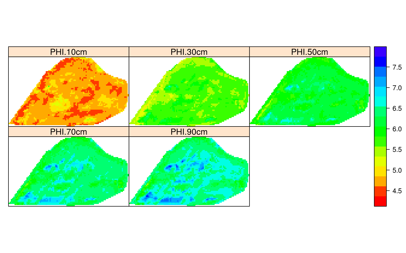
Figure 6.10: Predicted soil pH using 3D ensemble model.
The second prediction matrix can be used to determine model uncertainty:
library(matrixStats)
#>
#> Attaching package: 'matrixStats'
#> The following object is masked from 'package:plyr':
#>
#>     count
grid10m$PHI.10cm.sd <- rowSds(pred.PHI[[1]]$library.predict, na.rm=TRUE)
pts = list("sp.points", cookfarm.xy, pch="+", col="black", cex=1.4)
spplot(grid10m, "PHI.10cm.sd", sp.layout = list(pts), col.regions=rev(bpy.colors()))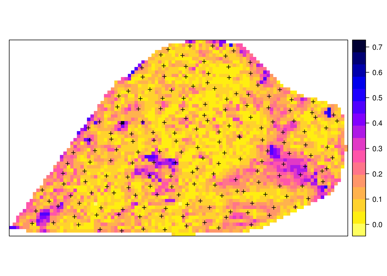
Figure 6.11: Example of variance of prediction models for soil pH.
which highlights the especially problematic areas, in this case most likely correlated with extrapolation in feature space. Before we stop computing, we need to close the cluster session by using:
stopCluster(cl)6.2 A generic framework for spatial prediction using Random Forest
We have seen, in the above examples, that MLA’s can be used efficiently to map soil properties and classes. Most currently used MLA’s, however, ignore the spatial locations of the observations and hence overlook any spatial autocorrelation in the data not accounted for by the covariates. Spatial auto-correlation, especially if it remains visible in the cross-validation residuals, indicates that the predictions are perhaps biased, and this is sub-optimal. To account for this, Hengl, Nussbaum, et al. (2018) describe a framework for using Random Forest (as implemented in the ranger package) in combination with geographical distances to sampling locations (which provide measures of relative spatial location) to fit models and predict values (RFsp).
6.2.1 General principle of RFsp
RF is, in essence, a non-spatial approach to spatial prediction, as the sampling locations and general sampling pattern are both ignored during the estimation of MLA model parameters. This can potentially lead to sub-optimal predictions and possibly systematic over- or under-prediction, especially where the spatial autocorrelation in the target variable is high and where point patterns show clear sampling bias. To overcome this problem Hengl, Nussbaum, et al. (2018) propose the following generic “RFsp” system:
\[\begin{equation} Y({{\bf s}}) = f \left( {{\bf X}_G}, {{\bf X}_R}, {{\bf X}_P} \right) \tag{6.1} \end{equation}\]where \({{\bf X}_G}\) are covariates accounting for geographical proximity and spatial relations between observations (to mimic spatial correlation used in kriging):
\[\begin{equation} {{\bf X}_G} = \left( d_{p1}, d_{p2}, \ldots , d_{pN} \right) \end{equation}\]where \(d_{pi}\) is the buffer distance (or any other complex proximity upslope/downslope distance, as explained in the next section) to the observed location \(pi\) from \({\bf s}\) and \(N\) is the total number of training points. \({{\bf X}_R}\) are surface reflectance covariates, i.e. usually spectral bands of remote sensing images, and \({{\bf X}_P}\) are process-based covariates. For example, the Landsat infrared band is a surface reflectance covariate, while the topographic wetness index and soil weathering index are process-based covariates. Geographic covariates are often smooth and reflect geometric composition of points, reflectance-based covariates can exhibit a significant amount of noise and usually provide information only about the surface of objects. Process-based covariates require specialized knowledge and rethinking of how to best represent processes. Assuming that the RFsp is fitted only using the \({\bf {X}_G}\), the predictions would resemble ordinary kriging (OK). If All covariates are used Eq. (6.1), RFsp would resemble regression-kriging (RK). Similar framework where distances to the center and edges of the study area and similar are used for prediction has been also proposed by T Behrens et al. (2018).
6.2.2 Geographical covariates
One of the key principles of geography is that “everything is related to everything else, but near things are more related than distant things” (Miller 2004). This principle forms the basis of geostatistics, which converts this rule into a mathematical model, i.e., through spatial autocorrelation functions or variograms. The key to making RF applicable to spatial statistics problems, therefore, lies also in preparing geographical (spatial) measures of proximity and connectivity between observations, so that spatial autocorrelation can be accounted for. There are multiple options for variables that quantify proximity and geographical connection (Fig. 6.12):
Geographical coordinates \(s_1\) and \(s_2\), i.e., easting and northing.
Euclidean distances to reference points in the study area. For example, distance to the center and edges of the study area, etc (T Behrens et al. 2018).
Euclidean distances to sampling locations, i.e., distances from observation locations. Here one buffer distance map can be generated per observation point or group of points. These are essentially the same distance measures as used in geostatistics.
Downslope distances, i.e., distances within a watershed: for each sampling point one can derive upslope/downslope distances to the ridges and hydrological network and/or downslope or upslope areas (Gruber and Peckham 2009). This requires, in addition to using a Digital Elevation Model, implementing a hydrological analysis of the terrain.
Resistance distances or weighted buffer distances, i.e., distances of the cumulative effort derived using terrain ruggedness and/or natural obstacles.
The gdistance package, for example, provides a framework to derive complex distances based on terrain complexity (van Etten 2017). Here additional inputs required to compute complex distances are the Digital Elevation Model (DEM) and DEM-derivatives, such as slope (Fig. 6.12b). SAGA GIS (Conrad et al. 2015) offers a wide variety of DEM derivatives that can be derived per location of interest.
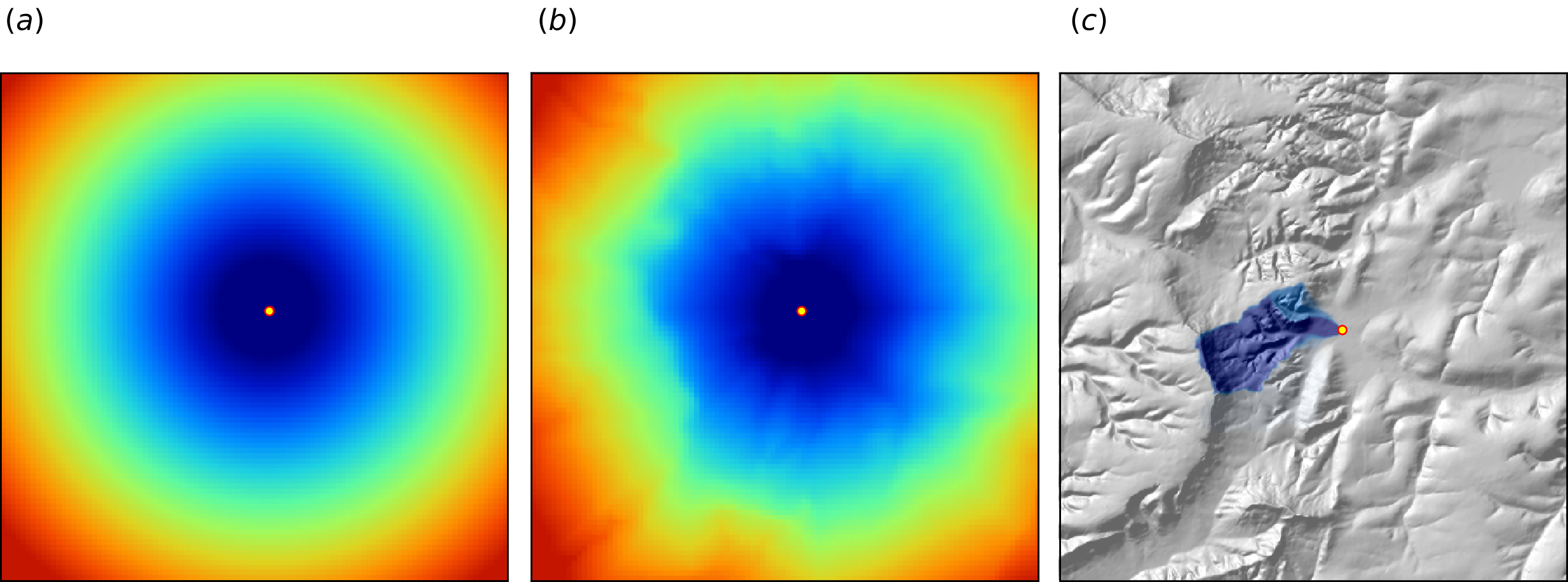
Figure 6.12: Examples of distance maps to some location in space (yellow dot) based on different derivation algorithms: (a) simple Euclidean distances, (b) complex speed-based distances based on the gdistance package and Digital Elevation Model (DEM), and (c) upslope area derived based on the DEM in SAGA GIS. Image source: Hengl et al. (2018) doi: 10.7717/peerj.5518.
Here, we only illustrate predictive performance using Euclidean buffer distances (to all sampling points), but the code could be adapted to include other families of geographical covariates (as shown in Fig. 6.12). Note also that RF tolerates a high number of covariates and multicolinearity (Biau and Scornet 2016), hence multiple types of geographical covariates (Euclidean buffer distances, upslope and downslope areas) could be considered concurrently.
6.2.3 Spatial prediction 2D continuous variable using RFsp
To run these examples, it is recommended to install ranger (Wright and Ziegler 2017) directly from github:
if(!require(ranger)){ devtools::install_github("imbs-hl/ranger") }Quantile regression random forest and derivation of standard errors using Jackknifing is available from ranger version >0.9.4. Other packages that we use here include:
library(GSIF)
library(rgdal)
#> rgdal: version: 1.3-6, (SVN revision 773)
#>  Geospatial Data Abstraction Library extensions to R successfully loaded
#>  Loaded GDAL runtime: GDAL 2.2.2, released 2017/09/15
#>  Path to GDAL shared files: /usr/share/gdal/2.2
#>  GDAL binary built with GEOS: TRUE
#>  Loaded PROJ.4 runtime: Rel. 4.8.0, 6 March 2012, [PJ_VERSION: 480]
#>  Path to PROJ.4 shared files: (autodetected)
#>  Linking to sp version: 1.3-1
library(raster)
library(geoR)
#> Warning: no DISPLAY variable so Tk is not available
#> --------------------------------------------------------------
#>  Analysis of Geostatistical Data
#>  For an Introduction to geoR go to http://www.leg.ufpr.br/geoR
#>  geoR version 1.7-5.2.1 (built on 2016-05-02) is now loaded
#> --------------------------------------------------------------
library(ranger)
#>
#> Attaching package: 'gridExtra'
#> The following object is masked from 'package:randomForest':
#>
#> combineIf no other information is available, we can use buffer distances to all points as covariates to predict values of some continuous or categorical variable in the RFsp framework. These can be derived with the help of the raster package (Hijmans and van Etten 2017). Consider for example the meuse data set from the sp package:
demo(meuse, echo=FALSE)We can derive buffer distance by using:
grid.dist0 <- GSIF::buffer.dist(meuse["zinc"], meuse.grid[1], as.factor(1:nrow(meuse)))which requires a few seconds, as it generates 155 individual gridded maps. The value of the target variable zinc can be now modeled as a function of these computed buffer distances:
dn0 <- paste(names(grid.dist0), collapse="+")
fm0 <- as.formula(paste("zinc ~ ", dn0))
fm0
#> zinc ~ layer.1 + layer.2 + layer.3 + layer.4 + layer.5 + layer.6 +
#>     layer.7 + layer.8 + layer.9 + layer.10 + layer.11 + layer.12 +
#>     layer.13 + layer.14 + layer.15 + layer.16 + layer.17 + layer.18 +
#>     layer.19 + layer.20 + layer.21 + layer.22 + layer.23 + layer.24 +
#>     layer.25 + layer.26 + layer.27 + layer.28 + layer.29 + layer.30 +
#>     layer.31 + layer.32 + layer.33 + layer.34 + layer.35 + layer.36 +
#>     layer.37 + layer.38 + layer.39 + layer.40 + layer.41 + layer.42 +
#>     layer.43 + layer.44 + layer.45 + layer.46 + layer.47 + layer.48 +
#>     layer.49 + layer.50 + layer.51 + layer.52 + layer.53 + layer.54 +
#>     layer.55 + layer.56 + layer.57 + layer.58 + layer.59 + layer.60 +
#>     layer.61 + layer.62 + layer.63 + layer.64 + layer.65 + layer.66 +
#>     layer.67 + layer.68 + layer.69 + layer.70 + layer.71 + layer.72 +
#>     layer.73 + layer.74 + layer.75 + layer.76 + layer.77 + layer.78 +
#>     layer.79 + layer.80 + layer.81 + layer.82 + layer.83 + layer.84 +
#>     layer.85 + layer.86 + layer.87 + layer.88 + layer.89 + layer.90 +
#>     layer.91 + layer.92 + layer.93 + layer.94 + layer.95 + layer.96 +
#>     layer.97 + layer.98 + layer.99 + layer.100 + layer.101 +
#>     layer.102 + layer.103 + layer.104 + layer.105 + layer.106 +
#>     layer.107 + layer.108 + layer.109 + layer.110 + layer.111 +
#>     layer.112 + layer.113 + layer.114 + layer.115 + layer.116 +
#>     layer.117 + layer.118 + layer.119 + layer.120 + layer.121 +
#>     layer.122 + layer.123 + layer.124 + layer.125 + layer.126 +
#>     layer.127 + layer.128 + layer.129 + layer.130 + layer.131 +
#>     layer.132 + layer.133 + layer.134 + layer.135 + layer.136 +
#>     layer.137 + layer.138 + layer.139 + layer.140 + layer.141 +
#>     layer.142 + layer.143 + layer.144 + layer.145 + layer.146 +
#>     layer.147 + layer.148 + layer.149 + layer.150 + layer.151 +
#>     layer.152 + layer.153 + layer.154 + layer.155
Subsequent analysis is similar to any regression analysis using the ranger package. First we overlay points and grids to create a regression matrix:
ov.zinc <- over(meuse["zinc"], grid.dist0)
rm.zinc <- cbind(meuse@data["zinc"], ov.zinc)
to estimate also the prediction error variance i.e. prediction intervals we set quantreg=TRUE which initiates the Quantile Regression RF approach (Meinshausen 2006):
m.zinc <- ranger(fm0, rm.zinc, quantreg=TRUE, num.trees=150, seed=1)
m.zinc
#> Ranger result
#>
#> Call:
#>  ranger(fm0, rm.zinc, quantreg = TRUE, num.trees = 150, seed = 1)
#>
#> Type:                             Regression
#> Number of trees:                  150
#> Sample size:                      155
#> Number of independent variables:  155
#> Mtry:                             12
#> Target node size:                 5
#> Variable importance mode:         none
#> Splitrule:                        variance
#> OOB prediction error (MSE):       67501
#> R squared (OOB):                  0.499
This shows that, using only buffer distance explains almost 50% of the variation in the target variable. To generate predictions for the zinc variable and using the RFsp model, we use:
q <- c((1-.682)/2, 0.5, 1-(1-.682)/2)
zinc.rfd <- predict(m.zinc, grid.dist0@data,
                    type="quantiles", quantiles=q)$predictions
str(zinc.rfd)
#>  num [1:3103, 1:3] 257 257 257 257 257 ...
#>  - attr(*, "dimnames")=List of 2
#>   ..$ : NULL
#>   ..$ : chr [1:3] "quantile= 0.159" "quantile= 0.5" "quantile= 0.841"
this will estimate 67% probability lower and upper limits and median value. Note that “median” can often be different from the “mean”, so, if you prefer to derive mean, then the quantreg=FALSE needs to be used as the Quantile Regression Forests approach can only derive median.
To be able to plot or export the predicted values as maps, we add them to the spatial pixels object:
meuse.grid$zinc_rfd = zinc.rfd[,2]
meuse.grid$zinc_rfd_range = (zinc.rfd[,3]-zinc.rfd[,1])/2
We can compare the RFsp approach with the model-based geostatistics approach (see e.g. geoR package), where we first decide about the transformation, then fit the variogram of the target variable (Diggle and Ribeiro Jr 2007; P. E. Brown 2015):
zinc.geo <- as.geodata(meuse["zinc"])
ini.v <- c(var(log1p(zinc.geo$data)),500)
zinc.vgm <- likfit(zinc.geo, lambda=0, ini=ini.v, cov.model="exponential")
#> kappa not used for the exponential correlation function
#> ---------------------------------------------------------------
#> likfit: likelihood maximisation using the function optim.
#> likfit: Use control() to pass additional
#>          arguments for the maximisation function.
#>         For further details see documentation for optim.
#> likfit: It is highly advisable to run this function several
#>         times with different initial values for the parameters.
#> likfit: WARNING: This step can be time demanding!
#> ---------------------------------------------------------------
#> likfit: end of numerical maximisation.
zinc.vgm
#> likfit: estimated model parameters:
#>       beta      tausq    sigmasq        phi
#> "  6.1553" "  0.0164" "  0.5928" "500.0001"
#> Practical Range with cor=0.05 for asymptotic range: 1498
#>
#> likfit: maximised log-likelihood = -1014
where likfit function fits a log-likelihood based variogram. Note that here we need to manually specify log-transformation via the lambda parameter. To generate predictions and kriging variance using geoR we run:
locs <- meuse.grid@coords
zinc.ok <- krige.conv(zinc.geo, locations=locs, krige=krige.control(obj.model=zinc.vgm))
#> krige.conv: model with constant mean
#> krige.conv: performing the Box-Cox data transformation
#> krige.conv: back-transforming the predicted mean and variance
#> krige.conv: Kriging performed using global neighbourhood
meuse.grid$zinc_ok <- zinc.ok$predict
meuse.grid$zinc_ok_range <- sqrt(zinc.ok$krige.var)
in this case geoR automatically back-transforms values to the original scale, which is a recommended feature. Comparison of predictions and prediction error maps produced using geoR (ordinary kriging) and RFsp (with buffer distances and using just coordinates) is given in Fig. 6.13.
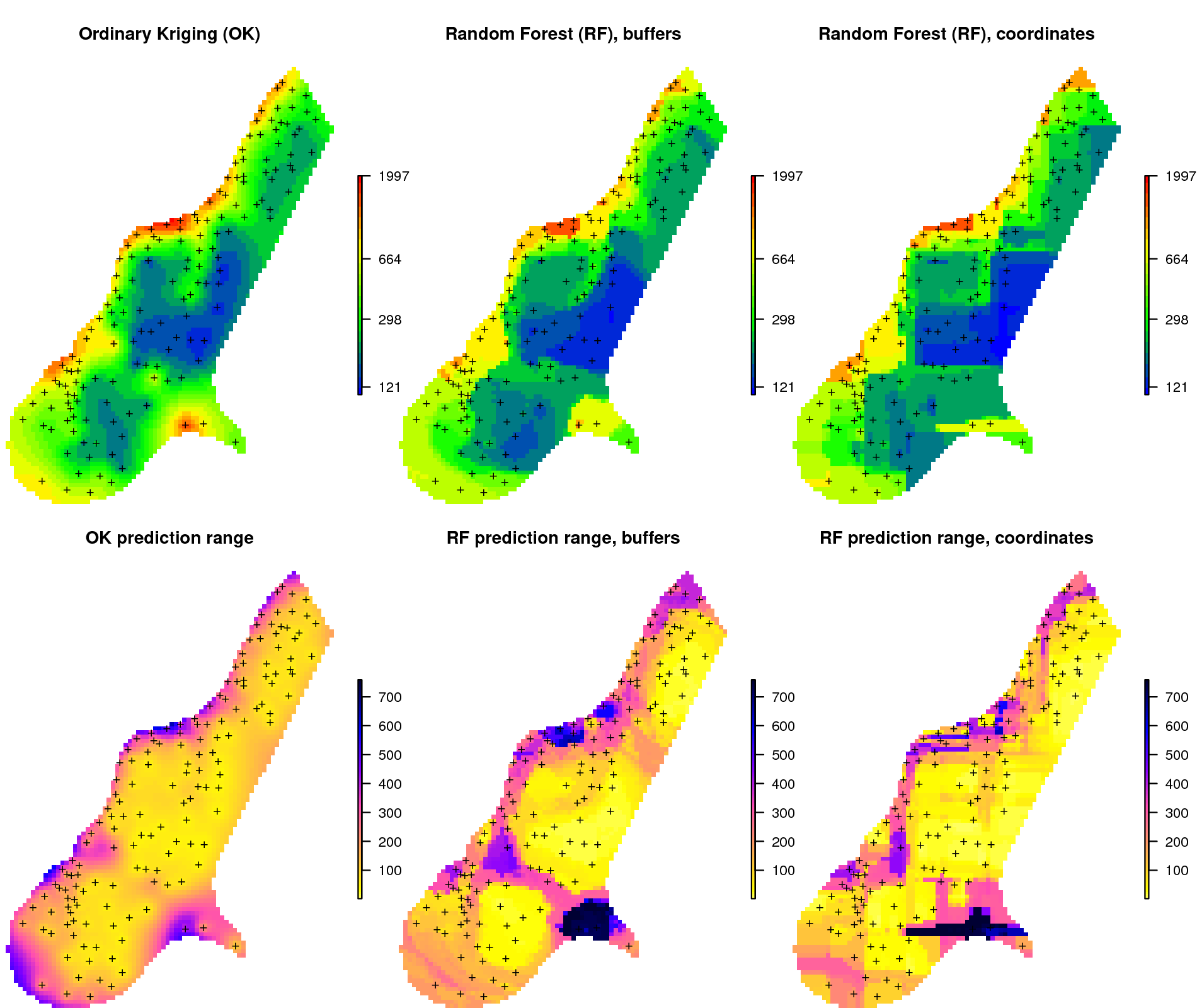
Figure 6.13: Comparison of predictions based on ordinary kriging as implemented in the geoR package (left) and random forest (right) for Zinc concentrations, Meuse data set: (first row) predicted concentrations in log-scale and (second row) standard deviation of the prediction errors for OK and RF methods. Image source: Hengl et al. (2018) doi: 10.7717/peerj.5518.
From the plot above, it can be concluded that RFsp yields very similar results to those produced using ordinary kriging via geoR. There are differences between geoR and RFsp, however. These are:
- RF requires no transformation i.e. works equally well with skewed and normally distributed variables; in general RF, requires fewer statistical assumptions than model-based geostatistics,
- RF prediction error variance on average shows somewhat stronger contrast than OK variance map i.e. it emphasizes isolated, less probable, local points much more than geoR,
- RFsp is significantly more computationally demanding as distances need to be derived from each sampling point to all new prediction locations,
- geoR uses global model parameters and, as such, prediction patterns are also relatively uniform, RFsp on the other hand (being tree-based) will produce patterns that match the data as much as possible.
6.2.4 Spatial prediction 2D variable with covariates using RFsp
Next, we can also consider adding additional covariates that describe soil forming processes or characteristics of the land to the list of buffer distances. For example, we can add covariates for surface water occurrence (Pekel et al. 2016) and elevation (AHN):
f1 = "extdata/Meuse_GlobalSurfaceWater_occurrence.tif"
f2 = "extdata/ahn.asc"
meuse.grid$SW_occurrence <- readGDAL(f1)$band1[meuse.grid@grid.index]
#> extdata/Meuse_GlobalSurfaceWater_occurrence.tif has GDAL driver GTiff
#> and has 104 rows and 78 columns
meuse.grid$AHN = readGDAL(f2)$band1[meuse.grid@grid.index]
#> extdata/ahn.asc has GDAL driver AAIGrid
#> and has 104 rows and 78 columns
to convert all covariates to numeric values and fill in all missing pixels we use Principal Component transformation:
grids.spc <- GSIF::spc(meuse.grid, as.formula("~ SW_occurrence + AHN + ffreq + dist"))
#> Converting ffreq to indicators...
#> Converting covariates to principal components...
so that we can fit a ranger model using both geographical covariates (buffer distances) and environmental covariates imported previously:
nms <- paste(names(grids.spc@predicted), collapse = "+")
fm1 <- as.formula(paste("zinc ~ ", dn0, " + ", nms))
fm1
#> zinc ~ layer.1 + layer.2 + layer.3 + layer.4 + layer.5 + layer.6 +
#>     layer.7 + layer.8 + layer.9 + layer.10 + layer.11 + layer.12 +
#>     layer.13 + layer.14 + layer.15 + layer.16 + layer.17 + layer.18 +
#>     layer.19 + layer.20 + layer.21 + layer.22 + layer.23 + layer.24 +
#>     layer.25 + layer.26 + layer.27 + layer.28 + layer.29 + layer.30 +
#>     layer.31 + layer.32 + layer.33 + layer.34 + layer.35 + layer.36 +
#>     layer.37 + layer.38 + layer.39 + layer.40 + layer.41 + layer.42 +
#>     layer.43 + layer.44 + layer.45 + layer.46 + layer.47 + layer.48 +
#>     layer.49 + layer.50 + layer.51 + layer.52 + layer.53 + layer.54 +
#>     layer.55 + layer.56 + layer.57 + layer.58 + layer.59 + layer.60 +
#>     layer.61 + layer.62 + layer.63 + layer.64 + layer.65 + layer.66 +
#>     layer.67 + layer.68 + layer.69 + layer.70 + layer.71 + layer.72 +
#>     layer.73 + layer.74 + layer.75 + layer.76 + layer.77 + layer.78 +
#>     layer.79 + layer.80 + layer.81 + layer.82 + layer.83 + layer.84 +
#>     layer.85 + layer.86 + layer.87 + layer.88 + layer.89 + layer.90 +
#>     layer.91 + layer.92 + layer.93 + layer.94 + layer.95 + layer.96 +
#>     layer.97 + layer.98 + layer.99 + layer.100 + layer.101 +
#>     layer.102 + layer.103 + layer.104 + layer.105 + layer.106 +
#>     layer.107 + layer.108 + layer.109 + layer.110 + layer.111 +
#>     layer.112 + layer.113 + layer.114 + layer.115 + layer.116 +
#>     layer.117 + layer.118 + layer.119 + layer.120 + layer.121 +
#>     layer.122 + layer.123 + layer.124 + layer.125 + layer.126 +
#>     layer.127 + layer.128 + layer.129 + layer.130 + layer.131 +
#>     layer.132 + layer.133 + layer.134 + layer.135 + layer.136 +
#>     layer.137 + layer.138 + layer.139 + layer.140 + layer.141 +
#>     layer.142 + layer.143 + layer.144 + layer.145 + layer.146 +
#>     layer.147 + layer.148 + layer.149 + layer.150 + layer.151 +
#>     layer.152 + layer.153 + layer.154 + layer.155 + PC1 + PC2 +
#>     PC3 + PC4 + PC5 + PC6
ov.zinc1 <- over(meuse["zinc"], grids.spc@predicted)
rm.zinc1 <- do.call(cbind, list(meuse@data["zinc"], ov.zinc, ov.zinc1))
this finally gives:
m1.zinc <- ranger(fm1, rm.zinc1, importance="impurity",
                  quantreg=TRUE, num.trees=150, seed=1)
m1.zinc
#> Ranger result
#>
#> Call:
#>  ranger(fm1, rm.zinc1, importance = "impurity", quantreg = TRUE,      num.trees = 150, seed = 1)
#>
#> Type:                             Regression
#> Number of trees:                  150
#> Sample size:                      155
#> Number of independent variables:  161
#> Mtry:                             12
#> Target node size:                 5
#> Variable importance mode:         impurity
#> Splitrule:                        variance
#> OOB prediction error (MSE):       56350
#> R squared (OOB):                  0.582
which demonstrates that there is a slight improvement relative to using only buffer distances as covariates. We can further evaluate this model to see which specific points and covariates are most important for spatial predictions:
xl <- as.list(ranger::importance(m1.zinc))
par(mfrow=c(1,1),oma=c(0.7,2,0,1), mar=c(4,3.5,1,0))
plot(vv <- t(data.frame(xl[order(unlist(xl), decreasing=TRUE)[10:1]])), 1:10,
     type = "n", ylab = "", yaxt = "n", xlab = "Variable Importance (Node Impurity)",
     cex.axis = .7, cex.lab = .7)
abline(h = 1:10, lty = "dotted", col = "grey60")
points(vv, 1:10)
axis(2, 1:10, labels = dimnames(vv)[[1]], las = 2, cex.axis = .7)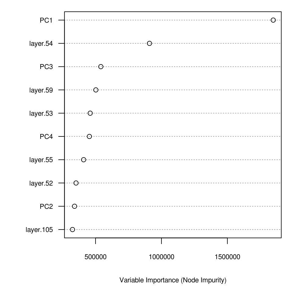
Figure 6.14: Variable importance plot for mapping zinc content based on the Meuse data set.
which shows, for example, that locations 54, 59 and 53 are the most influential points, and these are almost equally as important as the environmental covariates (PC2–PC4).
This type of modeling can be best compared to using Universal Kriging or Regression-Kriging in the geoR package:
zinc.geo$covariate = ov.zinc1
sic.t = ~ PC1 + PC2 + PC3 + PC4 + PC5
zinc1.vgm <- likfit(zinc.geo, trend = sic.t, lambda=0,
                    ini=ini.v, cov.model="exponential")
#> kappa not used for the exponential correlation function
#> ---------------------------------------------------------------
#> likfit: likelihood maximisation using the function optim.
#> likfit: Use control() to pass additional
#>          arguments for the maximisation function.
#>         For further details see documentation for optim.
#> likfit: It is highly advisable to run this function several
#>         times with different initial values for the parameters.
#> likfit: WARNING: This step can be time demanding!
#> ---------------------------------------------------------------
#> likfit: end of numerical maximisation.
zinc1.vgm
#> likfit: estimated model parameters:
#>      beta0      beta1      beta2      beta3      beta4      beta5
#> "  5.6929" " -0.4351" "  0.0002" " -0.0791" " -0.0485" " -0.3725"
#>      tausq    sigmasq        phi
#> "  0.0566" "  0.1992" "499.9990"
#> Practical Range with cor=0.05 for asymptotic range: 1498
#>
#> likfit: maximised log-likelihood = -980
this time geostatistical modeling produces an estimate of beta (regression coefficients) and variogram parameters (all estimated at once). Predictions using this Universal Kriging model can be generated by:
KC = krige.control(trend.d = sic.t,
                   trend.l = ~ grids.spc@predicted$PC1 +
                     grids.spc@predicted$PC2 + grids.spc@predicted$PC3 +
                     grids.spc@predicted$PC4 + grids.spc@predicted$PC5,
                   obj.model = zinc1.vgm)
zinc.uk <- krige.conv(zinc.geo, locations=locs, krige=KC)
#> krige.conv: model with mean defined by covariates provided by the user
#> krige.conv: performing the Box-Cox data transformation
#> krige.conv: back-transforming the predicted mean and variance
#> krige.conv: Kriging performed using global neighbourhood
meuse.grid$zinc_UK = zinc.uk$predict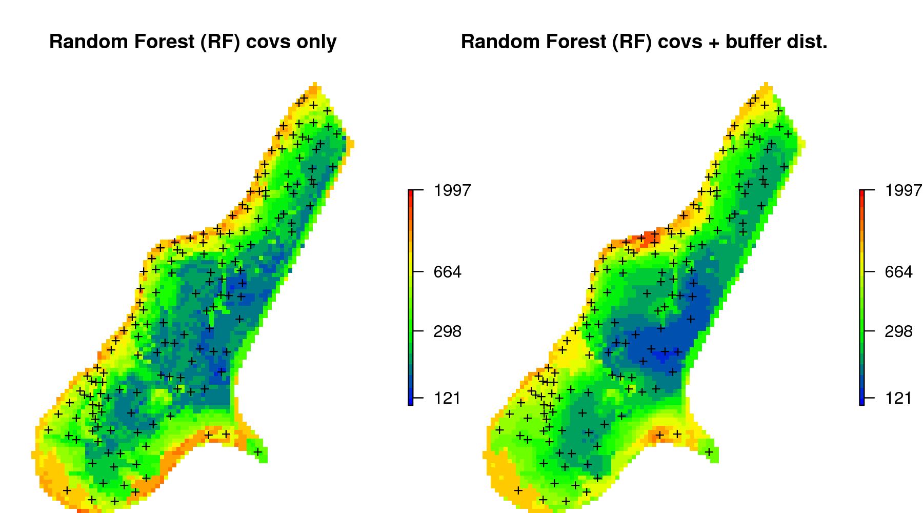
Figure 6.15: Comparison of predictions (median values) produced using random forest and covariates only (left), and random forest with combined covariates and buffer distances (right).
again, overall predictions (the spatial patterns) look fairly similar (Fig. 6.15). The difference between using geoR and RFsp is that, in the case of RFsp, there are fewer choices and fewer assumptions required. Also, RFsp permits the relationship between covariates and geographical distances to be fitted concurrently. This makes RFsp, in general, less cumbersome than model-based geostatistics, but then also more of a “black-box” system to a geostatistician.
6.2.5 Spatial prediction of binomial variables
RFsp can also be used to predict (map the distribution of) binomial variables i.e. variables having only two states (TRUE or FALSE). In the model-based geostatistics equivalent methods are indicator kriging and similar. Consider for example soil type 1 from the meuse data set:
meuse@data = cbind(meuse@data, data.frame(model.matrix(~soil-1, meuse@data)))
summary(as.factor(meuse$soil1))
#>  0  1
#> 58 97
in this case class soil1 is the dominant soil type in the area. To produce a map of soil1 using RFsp we have now two options:
- Option 1: treat the binomial variable as numeric variable with 0 / 1 values (thus a regression problem),
- Option 2: treat the binomial variable as a factor variable with a single class (thus a classification problem),
In the case of Option 1, we model soil1 as:
fm.s1 <- as.formula(paste("soil1 ~ ", paste(names(grid.dist0), collapse="+"),
                         " + SW_occurrence + dist"))
rm.s1 <- do.call(cbind, list(meuse@data["soil1"],
                             over(meuse["soil1"], meuse.grid),
                             over(meuse["soil1"], grid.dist0)))
m1.s1 <- ranger(fm.s1, rm.s1, mtry=22, num.trees=150, seed=1, quantreg=TRUE)
m1.s1
#> Ranger result
#>
#> Call:
#>  ranger(fm.s1, rm.s1, mtry = 22, num.trees = 150, seed = 1, quantreg = TRUE)
#>
#> Type:                             Regression
#> Number of trees:                  150
#> Sample size:                      155
#> Number of independent variables:  157
#> Mtry:                             22
#> Target node size:                 5
#> Variable importance mode:         none
#> Splitrule:                        variance
#> OOB prediction error (MSE):       0.0579
#> R squared (OOB):                  0.754
which results in a model that explains about 75% of variability in the soil1 values.
We set quantreg=TRUE so that we can also derive lower and upper prediction
intervals following the quantile regression random forest (Meinshausen 2006).
In the case of Option 2, we treat the binomial variable as a factor variable:
fm.s1c <- as.formula(paste("soil1c ~ ",
                           paste(names(grid.dist0), collapse="+"),
                           " + SW_occurrence + dist"))
rm.s1$soil1c = as.factor(rm.s1$soil1)
m2.s1 <- ranger(fm.s1c, rm.s1, mtry=22, num.trees=150, seed=1,
                probability=TRUE, keep.inbag=TRUE)
m2.s1
#> Ranger result
#>
#> Call:
#>  ranger(fm.s1c, rm.s1, mtry = 22, num.trees = 150, seed = 1, probability = TRUE,      keep.inbag = TRUE)
#>
#> Type:                             Probability estimation
#> Number of trees:                  150
#> Sample size:                      155
#> Number of independent variables:  157
#> Mtry:                             22
#> Target node size:                 10
#> Variable importance mode:         none
#> Splitrule:                        gini
#> OOB prediction error (Brier s.):  0.0586
which shows that the Out of Bag prediction error (classification error) is (only)
0.06 (in the probability scale). Note that, it is not easy to compare the results
of the regression and classification OOB errors as these are conceptually different.
Also note that we turn on keep.inbag = TRUE so that ranger can estimate the
classification errors using the Jackknife-after-Bootstrap method (Wager, Hastie, and Efron 2014).
quantreg=TRUE obviously would not work here since it is a classification and not a regression problem.
To produce predictions using the two options we use:
pred.regr <- predict(m1.s1, cbind(meuse.grid@data, grid.dist0@data), type="response")
pred.clas <- predict(m2.s1, cbind(meuse.grid@data, grid.dist0@data), type="se")
in principle, the two options to predicting the distribution of the binomial variable are mathematically equivalent and should lead to the same predictions (also shown in the map below). In practice, there can be some small differences in numbers, due to rounding effect or random start effects.
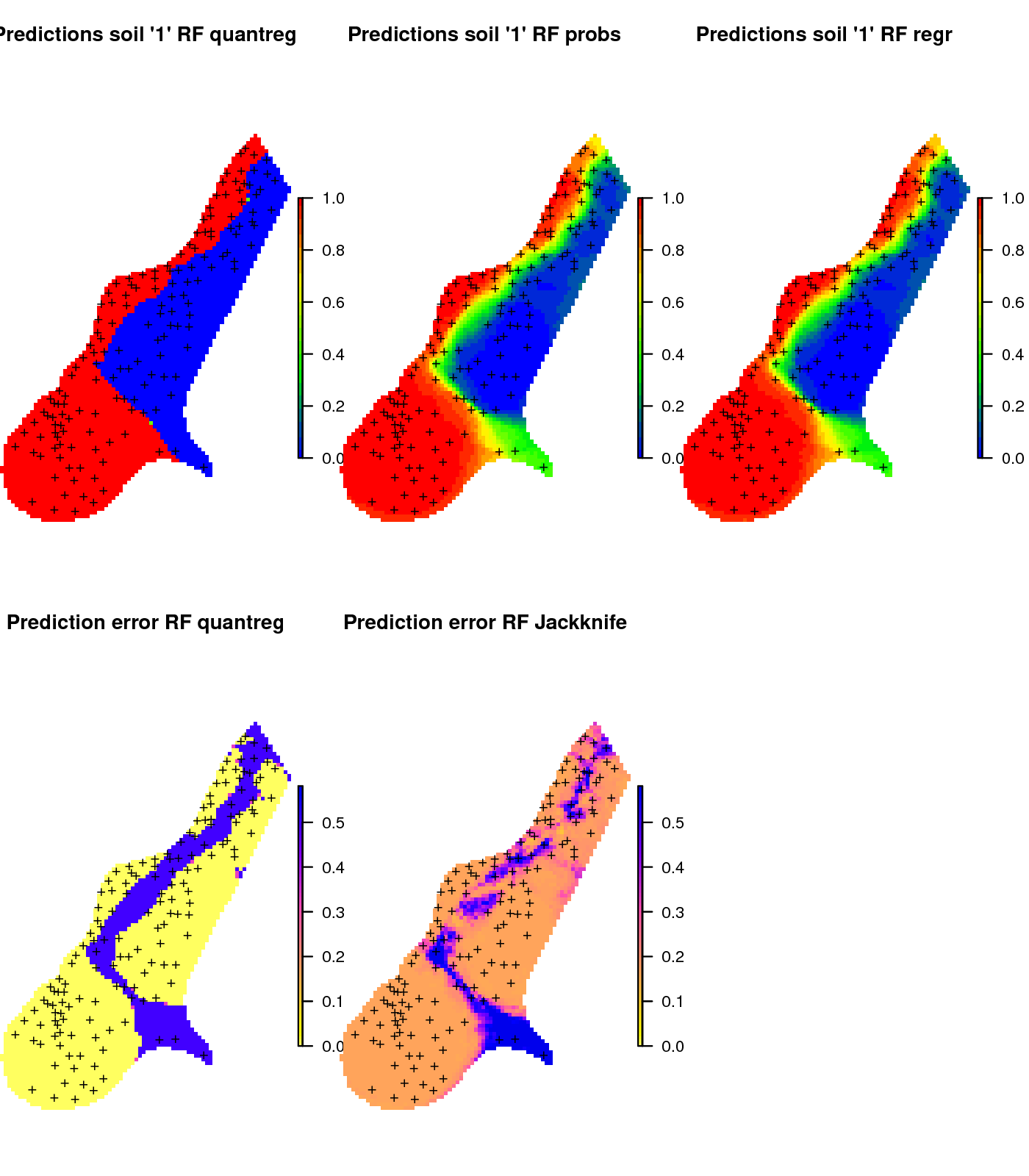
Figure 6.16: Comparison of predictions for soil class “1” produced using (left) regression and prediction of the median value, (middle) regression and prediction of response value, and (right) classification with probabilities.
This shows that predicting binomial variables using RFsp can be implemented both as a classification and a regression problem and both are possible to implement using the ranger package and both should lead to relatively the same results.
6.2.6 Spatial prediction of soil types
Spatial prediction of a categorical variable using ranger is a form of classification problem. The target variable contains multiple states (3 in this case), but the model still follows the same formulation:
fm.s = as.formula(paste("soil ~ ", paste(names(grid.dist0), collapse="+"),
                        " + SW_occurrence + dist"))
fm.s
#> soil ~ layer.1 + layer.2 + layer.3 + layer.4 + layer.5 + layer.6 +
#>     layer.7 + layer.8 + layer.9 + layer.10 + layer.11 + layer.12 +
#>     layer.13 + layer.14 + layer.15 + layer.16 + layer.17 + layer.18 +
#>     layer.19 + layer.20 + layer.21 + layer.22 + layer.23 + layer.24 +
#>     layer.25 + layer.26 + layer.27 + layer.28 + layer.29 + layer.30 +
#>     layer.31 + layer.32 + layer.33 + layer.34 + layer.35 + layer.36 +
#>     layer.37 + layer.38 + layer.39 + layer.40 + layer.41 + layer.42 +
#>     layer.43 + layer.44 + layer.45 + layer.46 + layer.47 + layer.48 +
#>     layer.49 + layer.50 + layer.51 + layer.52 + layer.53 + layer.54 +
#>     layer.55 + layer.56 + layer.57 + layer.58 + layer.59 + layer.60 +
#>     layer.61 + layer.62 + layer.63 + layer.64 + layer.65 + layer.66 +
#>     layer.67 + layer.68 + layer.69 + layer.70 + layer.71 + layer.72 +
#>     layer.73 + layer.74 + layer.75 + layer.76 + layer.77 + layer.78 +
#>     layer.79 + layer.80 + layer.81 + layer.82 + layer.83 + layer.84 +
#>     layer.85 + layer.86 + layer.87 + layer.88 + layer.89 + layer.90 +
#>     layer.91 + layer.92 + layer.93 + layer.94 + layer.95 + layer.96 +
#>     layer.97 + layer.98 + layer.99 + layer.100 + layer.101 +
#>     layer.102 + layer.103 + layer.104 + layer.105 + layer.106 +
#>     layer.107 + layer.108 + layer.109 + layer.110 + layer.111 +
#>     layer.112 + layer.113 + layer.114 + layer.115 + layer.116 +
#>     layer.117 + layer.118 + layer.119 + layer.120 + layer.121 +
#>     layer.122 + layer.123 + layer.124 + layer.125 + layer.126 +
#>     layer.127 + layer.128 + layer.129 + layer.130 + layer.131 +
#>     layer.132 + layer.133 + layer.134 + layer.135 + layer.136 +
#>     layer.137 + layer.138 + layer.139 + layer.140 + layer.141 +
#>     layer.142 + layer.143 + layer.144 + layer.145 + layer.146 +
#>     layer.147 + layer.148 + layer.149 + layer.150 + layer.151 +
#>     layer.152 + layer.153 + layer.154 + layer.155 + SW_occurrence +
#>     dist
to produce probability maps per soil class, we need to turn on the probability=TRUE option:
rm.s <- do.call(cbind, list(meuse@data["soil"],
                            over(meuse["soil"], meuse.grid),
                            over(meuse["soil"], grid.dist0)))
m.s <- ranger(fm.s, rm.s, mtry=22, num.trees=150, seed=1,
              probability=TRUE, keep.inbag=TRUE)
m.s
#> Ranger result
#>
#> Call:
#>  ranger(fm.s, rm.s, mtry = 22, num.trees = 150, seed = 1, probability = TRUE,      keep.inbag = TRUE)
#>
#> Type:                             Probability estimation
#> Number of trees:                  150
#> Sample size:                      155
#> Number of independent variables:  157
#> Mtry:                             22
#> Target node size:                 10
#> Variable importance mode:         none
#> Splitrule:                        gini
#> OOB prediction error (Brier s.):  0.0922
this shows that the model is successful with an OOB prediction error of about 0.09. This number is rather abstract so we can also check the actual classification accuracy using hard classes:
m.s0 <- ranger(fm.s, rm.s, mtry=22, num.trees=150, seed=1)
m.s0
#> Ranger result
#>
#> Call:
#>  ranger(fm.s, rm.s, mtry = 22, num.trees = 150, seed = 1)
#>
#> Type:                             Classification
#> Number of trees:                  150
#> Sample size:                      155
#> Number of independent variables:  157
#> Mtry:                             22
#> Target node size:                 1
#> Variable importance mode:         none
#> Splitrule:                        gini
#> OOB prediction error:             10.32 %
which shows that the classification or mapping accuracy for hard classes is about 90%. We can produce predictions of probabilities per class by running:
pred.soil_rfc = predict(m.s, cbind(meuse.grid@data, grid.dist0@data), type="se")
pred.grids = meuse.grid["soil"]
pred.grids@data = do.call(cbind, list(pred.grids@data,
                                      data.frame(pred.soil_rfc$predictions),
                                      data.frame(pred.soil_rfc$se)))
names(pred.grids) = c("soil", paste0("pred_soil", 1:3), paste0("se_soil", 1:3))
str(pred.grids@data)
#> 'data.frame':    3103 obs. of  7 variables:
#>  $ soil      : Factor w/ 3 levels "1","2","3": 1 1 1 1 1 1 1 1 1 1 ...
#>  $ pred_soil1: num  0.716 0.713 0.713 0.693 0.713 ...
#>  $ pred_soil2: num  0.246 0.256 0.256 0.27 0.256 ...
#>  $ pred_soil3: num  0.0374 0.0307 0.0307 0.0374 0.0307 ...
#>  $ se_soil1  : num  0.1798 0.1684 0.1684 0.0903 0.1684 ...
#>  $ se_soil2  : num  0.1446 0.0808 0.0808 0.0796 0.0808 ...
#>  $ se_soil3  : num  0.0414 0.0413 0.0413 0.0414 0.0413 ...
where pred_soil1 is the probability of occurrence of class 1 and se_soil1 is the standard error of prediction for the pred_soil1 based on the Jackknife-after-Bootstrap method (Wager, Hastie, and Efron 2014). The first column in pred.grids contains the existing map of soil with hard classes only.
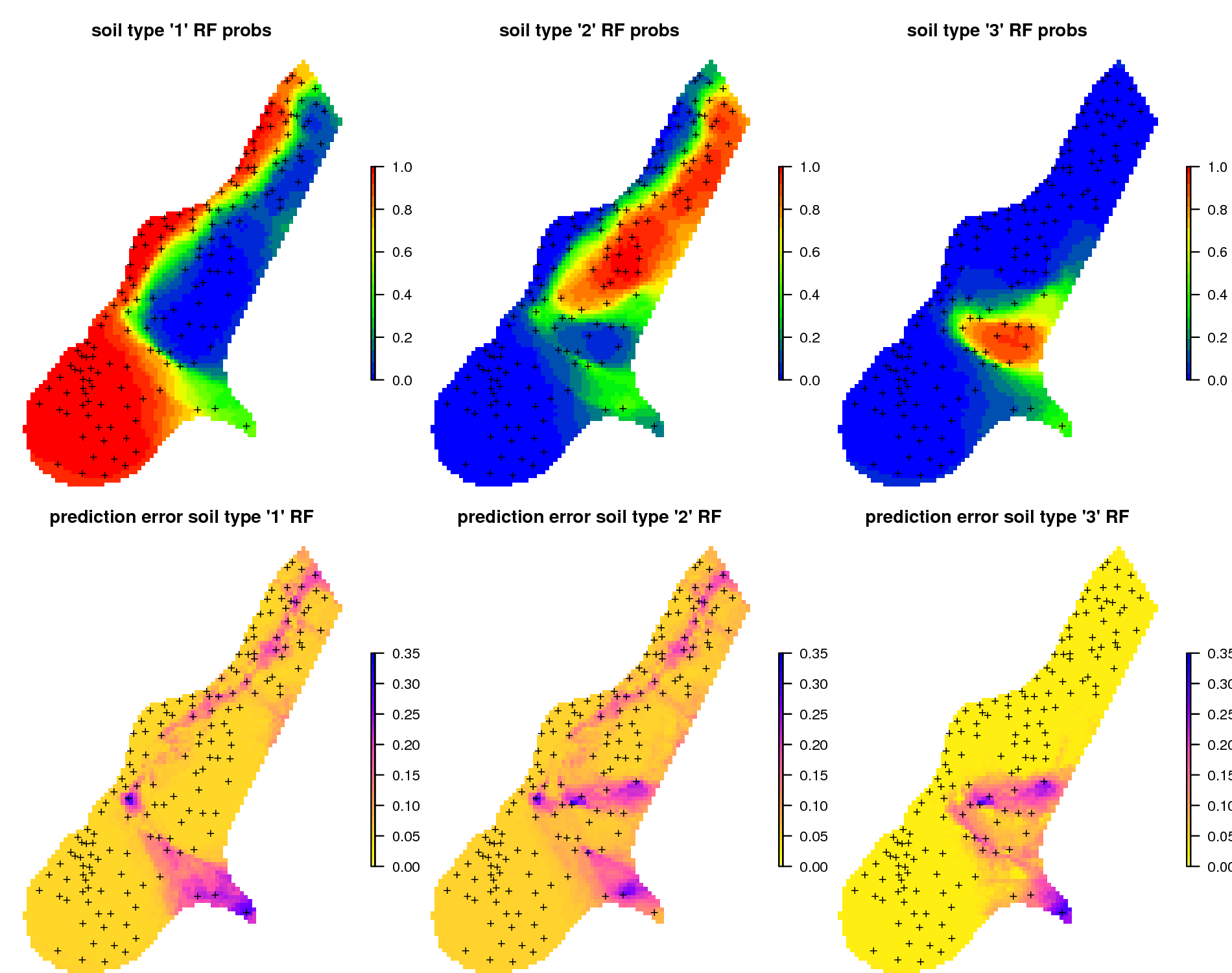
Figure 6.17: Predictions of soil types for the meuse data set based on the RFsp: (above) probability for three soil classes, and (below) derived standard errors per class.
Spatial prediction of binomial and factor-type variables is straightforward with ranger / RFsp: buffer distance and spatial-autocorrelation can be incorporated simultaneously as opposed to geostatistical packages, where link functions and/or indicator kriging would need to be used, and which require that variograms are fitted per class.
6.3 Summary points
In summary, MLA’s represent an increasingly attractive option for soil mapping and soil modelling problems in general, as they often perform better than standard linear models (as previously recognized by Moran and Bui (2002) and Henderson et al. (2004)) Some recent comparisons of MLA’s performance for operational soil mapping can be found in Nussbaum et al. (2018)). MLA’s often perform better than linear techniques for soil mapping; possibly for the following three reasons:
Non-linear relationships between soil forming factors and soil properties can be more efficiently modeled using MLA’s,
Tree-based MLA’s (random forest, gradient boosting, cubist) are suitable for representing local soil-landscape relationships, nested within a hierarchy of larger areas, which is often important for achieving accuracy of spatial prediction models,
In the case of MLA, statistical properties such as multicolinearity and non-Gaussian distribution are dealt with inside the models, which simplifies statistical modeling steps,
On the other hand, MLA’s can be computationally very intensive and consequently require careful planning, especially when the number of points goes beyond a few thousand and the number of covariates beyond a dozen. Note also that some MLA’s, such as for example Support Vector Machines (SVM), are computationally very intensive and are probably not well suited for very large data sets.
Within PSM, there is increasing interest in doing ensemble predictions, model averages or model stacks. Stacking models can improve upon individual best techniques, achieving improvements of up to 30%, with the additional demands consisting of only higher computation loads (Michailidis 2017). In the example above, the extensive computational load from derivation of models and product predictions already achieved improved accuracies, making increasing computing loads further a matter of diminishing returns. Some interesting Machine Learning Algorithms for soil mapping based on regression include: Random Forest (Biau and Scornet 2016), Gradient Boosting Machine (GBM) (Hastie, Tibshirani, and Friedman 2009), Cubist (Kuhn et al. 2014), Generalized Boosted Regression Models (Ridgeway 2018), Support Vector Machines (Chang and Lin 2011), and the Extreme Gradient Boosting approach available via the xgboost package (Chen and Guestrin 2016). None of these techniques is universally recognized as the best spatial predictor for all soil variables. Instead, we recommend comparing MLA’s using robust cross-validation methods as explained above. Also combining MLA’s into ensemble predictions might not be beneficial in all situations. Less is better sometimes.
The RFsp method seems to be suitable for generating spatial and spatiotemporal predictions. Computing time, however, can be demanding and working with data sets with >1000 point locations (hence 1000+ buffer distance maps) is probably not yet feasible or recommended. Also cross-validation of accuracy of predictions produced using RFsp needs to be implemented using leave-location-out CV to account for spatial autocorrelation in data. The key to the success of the RFsp framework might be the training data quality — especially quality of spatial sampling (to minimize extrapolation problems and any type of bias in data), and quality of model validation (to ensure that accuracy is not effected by over-fitting). For all other details about RFsp refer to Hengl, Nussbaum, et al. (2018).
References
Brungard, Colby W, Janis L Boettinger, Michael C Duniway, Skye A Wills, and Thomas C Edwards Jr. 2015. “Machine Learning for Predicting Soil Classes in Three Semi-Arid Landscapes.” Geoderma 239. Elsevier:68–83.
Heung, Brandon, Hung Chak Ho, Jin Zhang, Anders Knudby, Chuck E Bulmer, and Margaret G Schmidt. 2016. “An Overview and Comparison of Machine-Learning Techniques for Classification Purposes in Digital Soil Mapping.” Geoderma 265. Elsevier:62–77.
Behrens, Thorsten, Karsten Schmidt, Robert A MacMillan, and Raphael A Viscarra Rossel. 2018. “Multi-Scale Digital Soil Mapping with Deep Learning.” Scientific Reports 8 (October). Nature Publishing Group:15244. https://doi.org/10.1038/s41598-018-33516-6.
Richter, Aaron N, Taghi M Khoshgoftaar, Sara Landset, and Tawfiq Hasanin. 2015. “A Multi-Dimensional Comparison of Toolkits for Machine Learning with Big Data.” In Information Reuse and Integration (Iri), 2015 Ieee International Conference, 1–8. IEEE.
Sollich, Peter, and Anders Krogh. 1996. “Learning with Ensembles: How over-Fitting Can Be Useful.” In Advances in Neural Information Processing Systems, 8:190.
Kuhn, Max, Steve Weston, Chris Keefer, and Nathan Coulter. 2012. Cubist Models for Regression. https://cran.r-project.org/package=cubist.
Kuhn, Max, and Kjell Johnson. 2013. Applied Predictive Modeling. Vol. 810. Springer.
Chen, T., and C. Guestrin. 2016. “XGBoost: A Scalable Tree Boosting System.” ArXiv E-Prints, March.
Malone, B.P., A. B. McBratney, B. Minasny, and G.M. Laslett. 2009. “Mapping Continuous Depth Functions of Soil Carbon Storage and Available Water Capacity.” Geoderma 154 (1-2):138–52. https://doi.org/10.1016/j.geoderma.2009.10.007.
LeDell, Erin E. 2015. Scalable Ensemble Learning and Computationally Efficient Variance Estimation. University of California, Berkeley.
Gasch, Caley, Tomislav Hengl, Benedikt Gräler, Hanna Meyer, Troy Magney, and David Brown. 2015. “Spatio-temporal interpolation of soil water, temperature, and electrical conductivity in 3D+T: The Cook Agronomy Farm data set.” Spatial Statistics 14 (Part A):70–90. https://doi.org/10.1016/j.spasta.2015.04.001.
Polley, Eric C, and Mark J Van Der Laan. 2010. Super Learner in Prediction. Working Paper Series. U.C. Berkeley Division of Biostatistics.
Hengl, T., M. Nussbaum, M.N. Wright, G.B.M. Heuvelink, and B. Gräler. 2018. “Random Forest as a Generic Framework for Predictive Modeling of Spatial and Spatio-Temporal Variables.” PeerJ 6 (August):e5518. https://doi.org/10.7717/peerj.5518.
Behrens, T, K Schmidt, RA Viscarra Rossel, P Gries, T Scholten, and RA MacMillan. 2018. “Spatial modelling with Euclidean distance fields and machine learning.” European Journal of Soil Science 69 (5). Wiley Online Library:757–70.
Miller, Harvey J. 2004. “Tobler’s First Law and Spatial Analysis.” Annals of the Association of American Geographers 94 (2). Wiley Online Library:284–89.
Gruber, S., and S. Peckham. 2009. “Chapter 7 Land-Surface Parameters and Objects in Hydrology.” In Geomorphometry, edited by Tomislav Hengl and Hannes I. Reuter, 33:171–94. Developments in Soil Science. Elsevier. https://doi.org/10.1016/S0166-2481(08)00007-X.
van Etten, Jacob. 2017. “R Package gdistance: Distances and Routes on Geographical Grids.” Journal of Statistical Software 76 (13):1–21.
Conrad, O., B. Bechtel, M. Bock, H. Dietrich, E. Fischer, L. Gerlitz, J. Wehberg, V. Wichmann, and J. Böhner. 2015. “System for Automated Geoscientific Analyses (Saga) V. 2.1.4.” Geoscientific Model Development 8 (7). Copernicus GmbH:1991–2007. https://doi.org/10.5194/gmd-8-1991-2015.
Biau, Gérard, and Erwan Scornet. 2016. “A Random Forest Guided Tour.” TEST 25 (2). Springer:197–227. https://doi.org/10.1007/s11749-016-0481-7.
Wright, Marvin N, and Andreas Ziegler. 2017. “ranger: A Fast Implementation of Random Forests for High Dimensional Data in C++ and R.” Journal of Statistical Software 77 (1):1–17.
Hijmans, Robert J., and Jacob van Etten. 2017. Raster: Geographic Data Analysis and Modeling. http://CRAN.R-project.org/package=raster.
Meinshausen, Nicolai. 2006. “Quantile Regression Forests.” The Journal of Machine Learning Research 7 (Jun). JMLR.org:983–99.
Diggle, P. J., and P. J. Ribeiro Jr. 2007. Model-based Geostatistics. Springer Series in Statistics. Springer.
Brown, Patrick E. 2015. “Model-Based Geostatistics the Easy Way.” Journal of Statistical Software 63 (12). http://www.jstatsoft.org/v63/i12.
Pekel, Jean-François, Andrew Cottam, Noel Gorelick, and Alan S Belward. 2016. “High-Resolution Mapping of Global Surface Water and Its Long-Term Changes.” Nature 504. Nature Research:418–22.
Wager, Stefan, Trevor Hastie, and Bradley Efron. 2014. “Confidence Intervals for Random Forests: The Jackknife and the Infinitesimal Jackknife.” Journal of Machine Learning Research 15 (1):1625–51.
Moran, C.J., and E.N. Bui. 2002. “Spatial Data Mining for Enhanced Soil Map Modelling.” International Journal of Geographical Information Science 16 (6). Taylor & Francis:533–49.
Henderson, B. L., E. N. Bui, C. J. Moran, and D. A. P. Simon. 2004. “Australia-wide predictions of soil properties using decision trees.” Geoderma 124 (3-4):383–98.
Nussbaum, Madlene, Kay Spiess, Andri Baltensweiler, Urs Grob, Armin Keller, Lucie Greiner, Michael E Schaepman, and Andreas Papritz. 2018. “Evaluation of Digital Soil Mapping Approaches with Large Sets of Environmental Covariates.” Soil 4 (1):1.
Michailidis, Marios. 2017. “Investigating Machine Learning Methods in Recommender Systems.” PhD thesis, UCL (University College London).
Hastie, T.J., R.J. Tibshirani, and J.J.H. Friedman. 2009. The Elements of Statistical Learning: Data Mining, Inference, and Prediction. Springer Series in Statistics. Springer-Verlag New York.
Kuhn, Max, Steve Weston, Chris Keefer, Nathan Coulter, and R Quinlan. 2014. Cubist: Rule-and Instance-Based Regression Modeling. http://CRAN.R-project.org/package=Cubist.
Ridgeway, G. 2018. Gbm: Generalized Boosted Regression Models. http://CRAN.R-project.org/package=gbm.
Chang, Chih-Chung, and Chih-Jen Lin. 2011. “LIBSVM: a library for support vector machines.” ACM Transactions on Intelligent Systems and Technology (TIST) 2 (3). Acm:27.